WIXLIB

2Introductionthe intention of diversification. Allen (2010) argued that the mean-variance approach failedto diversify a portfolio in the 2008 financial crisis.There is an increasing need from both academic researchers and market practitioners forways of eligibly building more diversified portfolios. The new paradigm of portfolio allocation is the risk-based allocation strategy, which constructs a portfolio based solely on thevariance-covariance of assets. Examples of risk-based allocation strategies are minimumvariance (Behr et al., 2008; Clarke et al., 2006; Haugen and Baker, 1991), most diversifiedportfolio (Choueifaty and Coignard, 2008), risk parity (also known as the equal risk contribution) (Maillard et al., 2010; Qian, 2006) and diversified risk parity (Kind, 2013; Lohreet al., 2012, 2014) 1 .Two salient features of security investment are the uncertainty of security returns and thecorrelations between security returns. The correlations between securities, particularly lowor negative correlations, make diversification possible but it is also the reason the analysis ofsecurity investment is complicated. If there are only a few securities involved, for examplefive stocks, then it is easy and intuitive to simply look at the five variances and 10 correlations or covariances. However, if the number of securities is large, for example 200, it willnot be very helpful to simply look at the 200 variance and 19900 correlations or covariances.Principal component analysis (hereafter, PCA) is a statistical method of dimension reduction. It provides us with an alternative approach that is able to reduce the complexity - lookfor a few derived principal components that are designed to be uncorrelated while preserving most of the variation given by those variances and correlations or covariances (Jolliffe,1986). Although it has been widely used in many areas, until recently the studies applyingPCA to the finance sector were scarce, especially in the context of portfolio management.Our research focuses on the potential use of PCA in portfolio management. For simplicity, we study a portfolio only with stocks. There are two ways of applying PCA inconstructing portfolios. The PCA can reduce the complexity of a stock portfolio by transforming the stocks into a new set of uncorrelated principal components that represent uncor1 The diversified risk parity is an allocation strategy based on principal component analysis.It relates to ourresearch on applying principal component analysis in constructing portfolios, which we will discuss in moredetail in Chapter 3

3related risk sources. Then, instead of constructing portfolio based on the underlying stocks,one can treat the principal components as individual investment assets and simply choosefrom them. Hence, the analysis required for portfolio selection is therefore simplified.The other approach is using a selected subset of stocks to replace the original full dataset. This relates to an old question that has been researched for decades - how many stocksare needed to diversify a portfolio? The traditional capital-asset pricing model (CAPM)required the purchase of a market portfolio that contains all risky assets, but essentially themarket portfolio can be achieved with a much smaller portfolio. PCA allows us to identifythe stocks that can be used as a representative of the whole data set and therefore find thenumber of stocks that is sufficient to diversify a portfolio.Beside the use of PCA in portfolio construction, the most important application of PCAin portfolio management is to measure market concentration and the potential for diversification. While there are literatures which applied PCA to research market connectednessand argued that the diversification effects declined when the market was more concentrated,to the best of our knowledge no papers actually compare the degree of diversification to themarket connectedness. Moreover, to the best of our knowledge, no papers pointed out thatit is crucial to use the correlation matrix rather than the covariance matrix as input to a PCAwhen studying market connectedness. We research the problems associated with the useof covariance matrix and emphasize the importance of using the correlation matrix in thestudy.In many applications of PCA in finance, the high numbered principal components thatexplained little variance were normally discarded. No useful role was assigned to thoseprincipal components. But we found those components are effective in identifying nearlinearly correlated stocks.Our research is organized as below: Chapter 2 presents a brief description of principalcomponent analysis. Chapter 3 gives a literature review of relevant topics. Chapter 4 describes the data and methods. Chapter 5 determines the number of principal componentsrequired to represent the major risk sources in the stock market. Chapter 6 investigatesthe use of the high numbered principal components in identifying near linearly correlated

4Introductionstocks. Chapter 7 constructs portfolios based on the principal components retained in Chapter 5 and compares the equally weighted and equal risk contribution allocation strategies.Chapter 8 uses the principal component one to study the evolution of market connectedness over time. Chapter 9 investigates the time evolution of the relative importance of eachstock in the principal components retained in Chapter 5. Chapter 10 determines the numberof stocks are needed to make a diversified portfolio. Chapter 11 summaries the thesis anddiscusses potential further research.

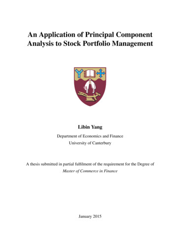
Chapter 2Principal component analysis: a briefreviewPrincipal Component Analysis (PCA) is a statistical method of dimension reduction that isused to reduce the complexity of a data set while minimizing information loss. It transformsa data set in which there are a large number of interrelated variables into a new set ofuncorrelated variables, the principal components, and which are ordered sequentially withthe first component explaining as much of the variation as it can. Each principal componentis a linear combination of the original variables in which the coefficients indicate the relativeimportance of the variable in the component.Consider an unrealistic, but simple, case of only two variables and the data are plottedin two dimensions. In Figure 2.1, we display the geometrical interpretation of the twovariable principal component analysis. The x1 and x2 represent the original variables andaxes. The PC1 and PC2 are the transformed variables and axes. The direction of the principalaxes indicates the principal components. The first principal component looks for a linearcombination α1′ x that explains the most variation, which isα1′ x α11 x1 α12 x2(2.1)where α1′ x is the eigenvalue of principle component one, x1 and x2 are the two original

6Principal component analysis: a brief reviewvariables, α1i is the coefficient of stock i in component one. Next, the principal componenttwo looks for a linear combination α2′ x that explains as much of the remaining variationconditional on it being orthogonal to principal component one. In a two variable case, thisis the remaining variation, which isα2′ x α21 x1 α22 x2(2.2)Clearly, in Figure 2.1 there is more variation in the direction of principal component one thaneither of the original variables, and leaves very little variation in the direction of principalcomponent two.PCA has often been treated as one special case of the factor analysis in textbooks. ButJolliffe (1986) stated that “this view is misguided since PCA and factor analysis, as usuallydefined, are really quite distinct techniques”. The PCA seeks to explain the diagonal termsof a covariance matrix or correlation matrix and also does a good job of explaining the offdiagonal terms. The factor analysis, on the other hand, seeks to explain the off-diagonalsterms but also explains the diagonal terms well. Moreover, both techniques aim to reducethe dimensionality of a data set (e.g. from a total of p variables) to a much smaller dimension m p. Changing m, the dimensionality of the model, can have much more dramaticeffects on factor analysis than it does on PCA. A final difference of these two techniques isthe principal component can be calculated exactly from the original variable, but the factorsin factor analysis cannot. Here we only provide a brief discussion of the principal component analysis just to help shape the basic understanding of this technique, for more detailedinformation, refer to Jolliffe (1986).

7Fig. 2.1 Geometric interpretation of principal component analysis (Graphic source http:// www.cheric.org/ ippage/ d/ ipdata/ 2014/ 01/ file/ d201401-401.pdf ).

Chapter 3Literature ReviewPCA is one of the best-known techniques in multivariate analysis. Its range of applicationshas expanded with the advent of computers and it has been used in a wide variety of areasfor the last 50 years (Jolliffe, 1986). The ability of PCA to decompose interrelated variablesinto uncorrelated components makes it attractive to use in analyzing the complex structureof financial markets. It has been applied to produce market indices (Feeney and Hester,1967) and to identify common factors in bond returns (Driesson et al., 2003; Pérignon et al.,2007). In more recent years, a growing literature applied PCA to the study of market crosscorrelation and systemic risk measurement (Billioand et al., 2012; Kritzman et al., 2011;Zheng et al., 2012). Most works have only discussed the theoretical framework of applyingPCA in portfolio management, few have actually looked into its performance. Our researchfocuses on the practical application of PCA to portfolio management. To the best of ourknowledge, no similar work has been done based on the Australian market.3.1Market connectedness and systemic riskSystemic risk is “the risk associated with the whole financial system, as opposed to anyindividual entity or component. It can be defined as any set of circumstance that threatensthe stability of financial system, and so potentially initiates financial crisis" (Zheng et al.,2012). The systemic risk is often misunderstood as the systematic risk. But they are in

10Literature Reviewfact different concepts. Systemic risk indicates the ratio of systematic risk to idiosyncraticrisk. An increase in the systemic risk suggests the proportion of systematic risk in thetotal risk increases. This means the amount of idiosyncratic risk, which is the diversifiablerisk, decreases. Conversely, an increase in systematic risk does not necessarily indicatea decrease in diversifiable risk. Consider when the amount systematic risk increases andthe idiosyncratic risk also increases while the ratio between them stays the same. So thesystemic risk was unchanged. The amount of diversifiable risk in this case increases ratherthan decreases.After the financial crisis in 2008, literature relating to systemic risk is substantial. Therehave been three groups of empirical studies on systemic risk. One of them focused on contagion, spillover effects and joint crashes in financial markets (Adrian, 2007; Billioand et al.,2012; Kritzman et al., 2011; Wang et al., 2011). Those studies were based on the analysis ofinterconnectedness among market security returns and our analysis on systemic risk followsin their steps. The other two groups of empirical studies on systemic risk include researchon the auto-correlation in the number of bank defaults, bank returns, and fund withdrawals(Brandt and Hartmann, 2000; Kenett et al., 2012; Lehar, 2005) and research on bank capitalratios and bank liabilities (Aguirre and Saidi, 2004; Bahansali et al., 2008; Brana and Lahet,2009) respectively. When the market becomes more connected, the systemic risk is higherin the sense that the negative shocks propagate more quickly and broadly. For this reason,monitoring the time evolution of correlation is critical. Moreover, low correlation betweenassets is what makes diversification possible, gaining insight into co-movement of securitiesis important in portfolio management.Other research has shown that the security correlations change in different time periods.Butler and Joaquin (2001) and Campbell et al. (2002) reported that the market correlationincreased in bear markets. Ferreira and Gama (2004), Hong et al. (2007), and Cappiello et al.(2006) reached the same conclusions for global industry returns, individual stock returns andinternational bond returns.Instead of comparing different time periods, many recent papers have applied PCA toinvestigate correlation using a sliding window approach. Fenn et al. (2011) applied PCA to

3.1 Market connectedness and systemic risk11study the evolution of correlation in a diverse range of asset classes: 25 developed marketequity indices, three emerging market indices, four corporate bond indices, 20 governmentbond indices, 15 currencies, nine metals, four fuel commodities, and 18 other commodities.They asserted that increases in the variance explained by the first component implied thatthere was more common variation in financial market. Moreover, they emphasized that thevariance explained by the first component might be the result of increases in the correlationsamong a few assets or a market-wide correlation. The first case will have less impact onthe diversification because one can simply move investments to less correlated assets. Incontrast, it becomes much more difficult to reduce risk by diversifying across different assetsif it is a market-wide correlation increase. They reported that the variance explained by thefirst principal component sharply increased when Lehman Brother filed for bankruptcy andMerrill Lynch agreed to be taken over by the Bank of America on 15 Sep 2008 was the caseof a market-wide correlation increase.Kritzman et al. (2011) introduced a measure of systemic risk called the absorption ratio.It is the fraction of variance absorbed by a finite number of principal components. They reported that most global financial crises were coincident with positive shifts of the absorptionratio. These crises include the Asian Financial Crisis in 1997, Russian default and LTCMcollapse in 1998, Housing bubble in mid-2006, and Lehman Brothers default in 2008. Another interesting finding in this paper is, in most cases, stock prices changed significantlywhen the absorption ratio reached its highest or lowest level.Zheng et al. (2012) not only looked at the absolute value of variance explained by thefirst component, they also computed the change in the variance explained to capture thesystemic risk. They obtained similar findings to Kritzman et al. (2011) that both the absolutevalue and change of variance explained by principal component one increased during afinancial crisis. But they reported that the moving window size and the time length used tocalculate the change had an impact on the date of the spike. The spike of absolute valueof variance explained by principal component one occurred later when the moving windowsize was larger and saturated after approximately 20-month time window. When the lengthof time used to calculate the change was longer, the change became delayed. While many

12Literature Reviewothers choose the size of moving window randomly, Zheng et al. (2012) pointed out thatthe size can impact the result. We believe that what Zheng et al. (2012) suggested is just amatter of sampling adequacy. One should not apply PCA to a data set that does not haveenough data points.3.2How many stocks make a diversified portfolio?Markowitz (1952)’s argued that instead of looking at single security alone, one should beconcerned with portfolios as a whole. The reason for this is that including securities thathave low correlations or even negative correlations could eliminate some risk. The existenceof many kinds of index funds provide means for investors to hold a diversified portfolio, butis it necessary to include all constituents within a index fund to obtain the same diversification as the index itself? Conventional wisdom has it that the benefits of diversification arevirtually exhausted when a portfolio contains a high enough number of stocks. However,how many stocks are enough remains an open question.Evans and Archer (1968) reported that approximately 10 randomly chosen stocks wouldbe adequate to diversify a portfolio. They observed that the benefit of diversification decreased as the number of stocks increased. Their conclusion has been cited in many textbooks (Francis, 1986; Gup, 1983; Reilly, 1985; Stevenson and Jennings, 1984). Newbouldand Poon (1993, 1996) followed Evans and Archer (1968)’s approach of comparing increasing size portfolio variance and claimed that just 8 to 20 stocks was enough to fully obtainthe benefit of diversification. However, Statman (1987) compared the cost and benefit ofdiversification and reported that the number of randomly chosen stocks that make a welldiversified portfolio was at least 30 using the data available in mid-1980s. Statman (2004)used the same approach and more available data, he then concluded that the break evenpoint, where the marginal benefit was equal to the marginal cost, exceeded 300 stocks.Subsequently, many others have reported different numbers of stocks needed to diversifya portfolio using risk measurements other than variance. Domian et al. (2003) reportedthat in order to avoid a significant shortfall risk, no less than 60 randomly chosen stocks

3.3 PCA in portfolio construction13were required. According to Domian et al. (2007), shortfall risk reduction continues as thenumber of randomly chosen stocks was increased, even above 100 stocks.The above researchers were using the number of stocks in a portfolio as a measure ofdiversification. However, this was problematic. If, in an ideal world, all stocks had samemean, variance and covariance, the number of stocks in a portfolio would be the key variable for estimating the reduction in variance (Frahm and Wiechers, 2011). In reality, suchassumptions do not hold. Intuitively, randomly choosing stocks to add to a portfolio, evenwhen they reach the number require

stock market. We constructed portfolio based on each of the ten principal components and named these "principal portfolios". Principal portfolio one, which represents the market risk, is essentially a 1/N portfolio on the underlying stocks, and principal portfolio two has the highest price correlation with the ASX200 index. Rebalancing the .