WIXLIB

442result, they typically have more success in actively managed funds that can react to theovercompensation and they trade better in trending markets rather than horizontal. Additionally,Bollinger Bands may be better suited for commodities trading or exchange rate trading, where “over 90%of them traders use technical analysis in their trading decisions” (Chen et al., 2014).An indicator %b tells where the moving average is within the bands. Unlike stochastic that arebounded by 0 and 100 %b can assume negative values and, values above 100, when prices areoutside of the bands. At 100, it is at the upper band, at 0 at the lower band, above 100, it is above theupper band and, below 0, and it is below the lower band (Bollinger, 1992).Bandwidth, another indicator derived from Bollinger Bands, may also interest traders. It is thewidth of the bands expressed as a percent of the moving average. When the bands narrow drastically,a sharp expansion in volatility usually occurs in the very near future (Bollinger, 1992).2.2. Trading rules of Bollinger BandsThe trading rules for the results of Bollinger Bands are illustrated as:Buy Rule: Closing Index (t) 𝐵𝐵𝑁𝐿 (t)Sell Rule: Closing Index (t) 𝐵𝐵𝑁𝑈 (t)A buy signal is generated when the closing index (price) crosses the lower band from below andthen a sell signal will be generated when the closing index (price) penetrates the upper band fromabove (William, 2006).One of the defining features is that they adjust in size which helps accounts for price volatilityaround the moving average. The bands tighten during times of higher stability and grow larger withhigher volatility (Kirkpatrick and Dahlquist, 2015).Other than the above strategies i.e. riding the bands, an investor can stay at the middle of thebands, i.e. at the point of 20-SMA and get out of the market. In other words, squeezing of the bandsforeshadows a big move to an investor. In addition to Bollinger Band, an investor should adopt thecandlestick chart to point out the double-top, double-bottom or, reversal trading strategy.2.3. Review of empirical studiesLeung and Chong (2003) compared the profitability of Moving Average Envelopes andBollinger Bands. Although Bollinger Bands can capture quick market fluctuations that MovingAverage Envelopes cannot, the study had shown that Bollinger Bands do not outperform MovingAverage Envelopes.Liu et al. (2006) found that the Black-Scholes stock price model has similar properties, that ofthe Bollinger Bands, i.e. widening when the market is volatile and vice versa. They came out with anew distribution of statistics, with the help of the concept of Bollinger Band.Lento and Gradojevic (2007) tested five different technical analysis tools S&P/TSX 300 Index,DJIA, NASDAQ Composite Index, and Canada and US spot exchange rate, and found that theBollinger Bands performed poorly and misleading the signals. They further found that even afteradjusting the transaction cost, the Bollinger Bands was not seen as highly profitable. Lento et al.(2007) applied the concept of Bollinger Bands, with variations in the moving average, on the threeleading stock markets and one foreign exchange trade, to see the informative effects in the market.They found that the Bollinger Bands are statistically inconsistent in producing better returns over theNational Accounting ReviewVolume 3, Issue 4, 439–451.

443buy-hold strategy. Similarly, Balsara et al. (2007) examined the random walk model and technicaltrading rules in Chinese stock markets namely, Shanghai and Shenzhen stock markets. They foundthat the Bollinger Bands breakout rule can bring out better return for an individual stock.Evans (2008) conducted the test on the S&P 500 data using Bollinger Bands basiccalculation, %b oscillators and concluded that a rotational trading algorithm using relative %brankings could select stock portfolios that beat the risk-adjusted return on the market.Kabansinskas and Macys (2010) looked at trading Bollinger Bands in the Baltic market toestablish the optimal parameters for the variables. As mentioned before, the value for N is 20, and Kis 2. However, the study looked at the ideal parameters for short-term, as well as, long-term investing.They concluded that for indicating short-term trends, N should be set to 10 and K to 1.9. Setting thevariables lower for short-term trading makes the metric more sensitive and, the security is moreprone to exceeding or dropping below the bounds, sending more trading signals. Decreasing Ndecreases the days in the average so, each day carries more weight in the SMA, and therefore, thestandard deviations. For long-term investing, they found the optimal parameters for N to be 50 and Kto be 2.1. This is opposite to the short-term trading variables by increasing the standard deviationsrequirements for a signal and therefore helps eliminate false signals.Kannan et al. (2010) adopted typical price, Chaikin money flow indicator, stochastic momentumindex, relative strength index, moving average, and Bollinger Bands to discover the predictingcapacity for the return from the stock market. They concluded that stochastic momentum, the besttool, followed by the Bollinger Bands with an accuracy of about 85 percent, gives a profitabilitysignal from the historical data of the stock market.Lee et al. (2013) constructed lower and upper bounds within which future values of thestochastic process run at a fixed probability level. During the short-selling of the stock, the boundsconstructed were termed as price-bands or trading-bands. In the paper, they came out with amathematical model for the construction of price bands using a stochastic programming formulation.Chen et al. (2014) used the GARCH (1,1) with Bollinger Bands to determine the distributionnature of the market return. The study found that the combination helped in producing a betterperformance for the results from the Bollinger Bands. Fang et al. (2014) found the results from theBollinger Band as a part of the trading strategy in most of the international stock markets with thegradually declining popularity after the year 2001. Similarly, Lim et al. (2014) looked at theprofitability of a trading rule based on Bollinger Bands in six different equity markets using large-capindices, namely; CAC, DAX, FTSE, HSI, KOSPI, and NIKKEI. Besides, they also explored theperformance of a trading strategy based on a combined signal approach with Bollinger Band signals;filtered using the ADX to avoid trending markets. They found evidence to support the use of BollingerBands for tactical trades over short time horizons, with a strong-positive skewed distribution for thereturns. When comparing the performance of Bollinger bands with the strategy augmented by the ADX,they found the low-performance improvement when applied on a systematic basis as an initial filter.However, they suggested applying the ADX on a discretionary basis to limit losses.In context to Indian listed companies, Shah and Patel (2015) found that the Bollinger Bandsoutperformed than Relative Strength Index (RSI) and SMA (Simple Moving Average) to find out thebuy and sell signals as well as profitability from specific security. Similarly, Pushpa et al. (2017)found that Bollinger Bands help to give a strong buy signal and sell signal with other technicalanalysis tools like SMA, MACD, and RSI.National Accounting ReviewVolume 3, Issue 4, 439–451.

444Similarly, Prasad et al. (2018) tested the volatility of the share prices of the six commercialbanks of India using the Bollinger Bands. Based on the widening and tightness of the upper andlower bands, the paper found only two sample banks with less volatility among the sampled banks.Chen et al. (2018) applied the concept of Bollinger Bands with wavelet analysis on stock indexfuture CSI 300 of China to determine the trading strategy for an investor with a greater return, lessrisky and, higher applicability. They found that the combination of Bollinger Bands with waveletanalysis prevents a false break during transactions.Khairi et al. (2019) found that technical analysis tools like stochastic oscillators, Moving AverageConvergent Divergent (MACD), Bollinger Bands (BB), and Relative Strength Index (RSI) were seensignificant in predicting the stock price trend for a shorter run only. Hence, to get an accurateprediction of the market trend, suitable fundamental analysis techniques, and machine learningtechniques helped an investor.Pramudya and Ichsani (2020) conducted a comparative study to determine the accuracy of buyand sell signals on the Indonesian stock market, IDX LQ45, provided by Moving AverageConvergent Divergent (MACD), Bollinger Bands, and Relative Strength Index (RSI). They foundthat the Bollinger Bands and the MACD indicators captured sell signals better than the RSI. Theyalso found that MACD was much slower to give a sell signal than the Bollinger Bands and,statistically significant RSI, thus an investor should be highly cautious in getting an accurate result.Mkik and Menzhi (2020) revealed that the Bollinger Bands is not profitable. The various signalsunder Bollinger Bands are consistently underperforming the buyer’s trading strategy and the hold.After adjusting for transit costs, the Bollinger Bands are only cost-effective for 2 out of 12 tests.Furthermore, no particular Bollinger Bands variant indicated robust and superior performance.Although the reason for the use of the BB oscillator (i.e., to sell when the market is overboughttainted when the market is oversold), when a contrary approach was used, the profitability of the BBhas been improved impressive (i.e., buy on a sell signal and sell on a buy signal).Ni et al. (2020) explored the Taiwan 50 whether an investor could beat the market by tradingwith the support of signals provided by the Bollinger Bands. The study revealed that the marketcould be beaten by taking a long position on stocks lying on the lower band, providing a significantlyabnormal profit. The study also found that an investor should take a long position when the pricereaches the upper band.Chandima (2021) stated that the Bollinger Bands are used for the volatility evaluation of thestock market. The study found that the squeezing of the bands signals the start of a new move in themarket. While testing the Bollinger Bands in Colombo Stock Exchange, the researcher found that thebands of Bollinger Bands could be viewed as support and resistance for the market. Similarly, Singhet al. (2021) found that the Bollinger Bands as a valuable tool for traders to measure volatilityposition and guide them into when to enter the market and leave a position.3.MethodologyThe paper has followed the exploratory research design, as it tries to find out the new andunexplored side of the use of one of the technical analysis tools, namely, Bollinger Bands in NepalStock Exchange Limited (NEPSE). For the data analysis purpose, the paper has used the dailyclosing index recorded in the only secondary market of Nepal Stock Exchange Limited (NEPSE).The daily NEPSE Index is calculated based on the amount of market capitalization during a specificNational Accounting ReviewVolume 3, Issue 4, 439–451.

445day. The daily indices have been considered of twenty-two (22) years from fiscal year (F/Y)1998–1999 to the fiscal year (F/Y) 2019–2020. The fiscal year in Nepal starts in mid-July accordingto the Georgian calendar.The paper initially calculated the 20-SMA for the daily NEPSE Index of the sample periods.Then, the Upper Bollinger Band (UBB) and Lower Bollinger Band (LBB) have been calculated asdefined by Bollinger (1992). The calculated value was then plotted to get a glimpse of the marketvolatility. Similarly, the value of %b (percent b) and Bollinger BWI (Bandwidth Index) wascalculated to determine the volatility signal from the NEPSE.Writing upper band for the upper Bollinger Band, lower band for the lower Bollinger Band, andclose for the closing (price) value:%b (Close Lower Band) / (Upper Band Lower Band)Bandwidth tells how wide the Bollinger Bands are on a normalized basis. Writing the samesymbols as before, and middle band for the moving average, or middle Bollinger Band:Bandwidth (Upper Band Lower Band)/Middle BandUsing the default parameters of a 20-period simple moving average and, plus/minus two (2)standard deviations, bandwidth is equal to four times the 20-period coefficient of variation(Bollinger, 2001).A popular indicator derived from the Bollinger Bands is the Bandwidth Indicator, BWI. It canbe calculated as:𝐵𝑊𝐼𝑡 𝑈𝐵𝑡𝛿 𝐿𝐵𝑡𝛿(1)𝑀𝐴𝛿𝑡where, 𝑈𝐵𝑡𝛿 Upper band at time “t” with a size of “ ”𝐿𝐵𝑡𝛿 Lower band at time “t” with a size of “ ”𝑀𝐴𝛿𝑡 Moving average for time “t” with a size of “ ”Similarly, the estimated density of Q or unimodality of Q can be calculated as:112𝑄 0 𝐵𝑠2 𝑑𝑠 ( 0 𝐵𝑠2 𝑑𝑠)(2)where, “Bs” is the Bandwidth indicator i.e. BWI.For the normal distribution or a unimodal distribution, a positive value of “Q” states the strongunimodality and for the negative value, vice-versa (Ibrahim, 2013).The concept of definite integral calculus has been followed for calculating the value of Q, whereintegral of “Bs” is from 1 to 0 and, the arbitrary constant “c” is absent. Here, 𝐵𝑠2 is called theintegrand, 1 is called the upper limit, and 0 is called the lower limit of integration.At the same time, the value of UBB and LBB were compared with the NEPSE Index (Closing)to determine the buy signal, sell signal, or no signal as defined by William (2006).4.Findings and results4.1. Diagrammatic presentation of UBB, LBB and SMAFigure 1 shows the movement of the Upper Bollinger Band (UBB) and Lower Bollinger Band(LBB) as well as Simple Moving Average (SMA). The figure will also help to state whether themarket is at a bullish trend or in the bearish trend. As the SMA line passes between the UBB andNational Accounting ReviewVolume 3, Issue 4, 439–451.

446LBB lines, the market can be stated as stable. But as the SMA line passes above the UBB, the trendmarket follows will be the bullish and vice-versa if passes below the LBB.Figure 1. NEPSE Index 20 Days SMA, LBB and UBB.At the same time, when the bands, i.e. UBB and LBB lie close together, a period of low volatilityis indicated. Conversely, as the bands expand, an increase in price action/market volatility is indicated.When the bands have only a slight slope and track approximately parallel for an extended time, theprice will generally be found to oscillate between the bands as though in a channel.The Figure 1 shows the band was tightly closed indicating low volatility (trading days of theyear 2001–2002 to 2004–2005) and at the same time, the low parallel which indicates no visiblemarket fluctuation. During this period only, the SMA is hardly moving between the UBB and LBB.When the LBB and UBB are seen parallel, the traders are interested to sell at the point of UBB andbuy at the point of LBB.The 20-SMA is seen closer to the UBB at the end of the year 2020 as the market closed with thebullish signal. Though, the market had shown the signal of high volatility, moving closer to lowerband most of the days or, being tighter between the bands.4.2. %b (Percent b)%b (pronounced “percent b”) is derived from the formula for Stochastic and shows where priceis in relation to the bands. %b equals “1” at the upper band and “0” at the lower band. The graphicalpresentation and the calculation value of %b is equal to the value 1 reflects the market is in bullishtrend and when the calculation value of %b is equal to the value 0 reflects the market is in bearishtrend. The result of the %b also helps to determine the market fluctuation is within the UBB andLBB of the Bollinger Band. Hence, it is used only for market pattern recognition. The figure belowshows the plotted value of %b for NEPSE.Under the Bollinger Band analysis, %b is one of the common indicators to see the where themarket price is being positioned during a specific time period. When the %b graph is highly dense atthe upper level, the market shows the bullish trend and vice-versa. In other words, if the graph movescloser to the value “1”, the market is seen in the bullish trend and if the graph moves closer to thevalue “0”, the market is seen in the bearish trend.National Accounting ReviewVolume 3, Issue 4, 439–451.

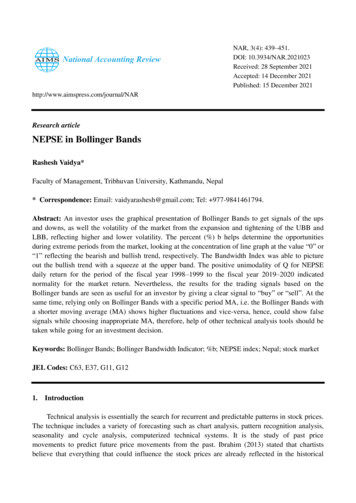
4471.00.8%b0.60.40.20.0Day (t)Figure 2. Value of %b.4.3. Bollinger Bandwidth Indicator (BWI)Bollinger Bandwidth Indicators (BWI) tells how wide the Bollinger Bands are on a normalizedbasis. It is the value of difference between the UBB and LBB divided by the MA for the specific timeperiod. The main motto of plotting the value of BWI is to capture the opportunities from theextremes in market volatility and trend identifications.6.5BWI.4.3.2.1.0Day (t)Figure 3. Bollinger Bandwidth Indicator (BWI).The BWI shows how the market is taking its movement. This shows how the upper-band andlower-band are moving in a normalized basis i.e. ups and downs of the market. If the BWI is seen highlyfluctuating, it can be stated that the market is ready for fluctuation. The market needs to show somefluctuation as it is a natural but abnormal fluctuation bring volatility to the market. If the BWI shows theregular squeezes at upper point, followed by a break, then the market tends to reflect the bullish trendand vice versa. A limited number of upper point extreme squeezes were seen during the study periodshowing few number bullish trends in NEPSE which ultimately brought volatility in the market.National Accounting ReviewVolume 3, Issue 4, 439–451.

4484.4. Unimodality of QFor the normal distribution, a positive value of “Q” states the strong unimodality and for thenegative value, vice-versa. Simply, unimodality of “Q” is the estimated density of the value “Q”.20Unimodality Q.16.12.08.04.00Day (t)Figure 4. Unimodality Q.Instead of the finding of 95% of the data inside the bands, as would be the expectation with thedefault parameters if the data were normally distributed, studies have found that only about 88% ofsecurity prices (85%–90%) remain within the bands. Thus, the unimodality of Q is being calculatedto see the exact distribution of the MA. As the values of unimodality of Q for the past twenty-twoyears are seen all positive, which state the strong unimodality for the NEPSE daily index.4.5. Trading signal from Bollinger BandsTable 1 shows the number of buy signals and sell signals shown by Bollinger Bands for NEPSE.Table 1. Trading signal from Bollinger Bands.DescriptionNumber of ObservationsTotal Trading Days4856Buy Signals437Sell Signals302Source: Annex.More number of strong “buy signals” was seen provided from the Bollinger Bands analysis forthe NEPSE than the “sell signals” during the observation period.A buy signal is generated when the closing index (price) crosses the lower band from below andthen a sell signal will be generated when the closing index (price) penetrates the upper band from above.This shows that the daily closing NEPSE index were at higher level than the lower Bollinger Bandsfor more time periods during the period of F/Y 1998–1999 to F/Y 2019–2020. The buy and sell signalsprovided from the Bollinger Bands, also helps an investor to determine an entry or an exit strategy.National Accounting ReviewVolume 3, Issue 4, 439–451.

4495.Conclusions and implicationsThe graphical plotting of the Upper Bollinger Band (UBB) and Lower Bollinger Band (LBB)with the 20-SMA or, 20-EMA helps to visualize the stock market volatility. As the UBB and LBBtighten closer, the stock market reflects lesser volatility and vice versa. The graphical presentation ofthe NEPSE Index (Daily Closing) reflected a short period of market volatility during the study periodof F/Y 1998–1999 to F/Y 2019–2020. The deviation in the Nepalese market from the upper andlower bands was so minimal, that the interpretation from the Bollinger Bands was not productive.The result from the %b (percent b) reflected the market trend for NEPSE. When the plottedgraph for the value of %b becomes denser at the value of “1”, it reflected bullish, and when the graphfor %b becomes denser at the value of “0”, it reflected the market is a bearish trend.The model developed for unimodality was put in question for its operational efficiency in thereal market. The

Bollinger (1992) discussed the envelope or trading bands that can provide the buying or selling signals to investors with the help of MA and deviation from the MA. The Bollinger Bands strategy does not chase momentum as by MA strategy, as it tries to recognize the point where either an upward trend or downward trend ends.