WIXLIB

COMP 4971 – Independent Study (Fall 2018/19)Optimization of Bollinger Bandson Trading Common StockMarket IndicesCHUI, Man Chun MartinYear 3, BSc in Biotechnology and BusinessSupervised By:Professor David ROSSITERDepartment of Computer Science and Engineering

Table of Contents1.Introduction . 31.1.Bollinger Bands . 31.2.Common Stock Market Indices to be Analysed . 42.Source of Data and Software Framework. 43.Algorithm Development . 54.3.1.Moving Average and Moving Standard Deviation Functions . 53.2.Exponentially Weighted Bollinger Bands . 73.3.Asymmetric Bollinger Bands . 93.4.Settings, Assumptions and Flow of the Trading Algorithm . 12Results and Discussions. 144.1.Performance Evaluation of the Algorithm in Short, Medium, and Long Terms . 144.1.1.Results of Trading on Hang Sang Index . 154.1.2.Results of Trading on S&P 500 . 184.1.3.Results of Trading on Nikkei 225 . 194.2.Suggested Strategies for Trading with Bollinger Bands . 215.Conclusion . 226.Reference . 227.Appendices . 231

Table of FiguresFigure 1 Bollinger Bands plotted by StockChart.com (top) and Stoxy (bottom) . 6Figure 2 Standard Bollinger Bands (green) and EW Bollinger Bands (blue). 8Figure 3 Notation of Buy and Sell Signals on Bollinger Bands . 9Figure 4 Bollinger Bands with 1.5 SD (green) and 2 SD (blue) away from 20-day SMA . 10Figure 5 Heatmaps of Return by Trading with Bollinger Bands . 11Figure 6 Excess Return for 3-Years Trading Test on Hang Sang Index . 16Figure 7 Excess Return for 3-Years Trading Test on S&P 500 . 18Figure 8 Excess Return for 3-Years Trading Test on Nikkei 225 . 19Figure 9 Historical Data of Hang Sang Index Plotted with 2 Suggested Bollinger Bands . 24Figure 10 Annual Return of 3-years Investments on Hang Sang Index from 2006 to 2018 . 25Figure 11 Historical Data of S&P 500 Plotted with 2 Suggested Bollinger Bands . 27Figure 12 Annual Return of 3-years Investments on S&P500 from 2006 to 2018. 28Figure 13 Historical Data of Nikkei 225 Plotted with 2 Suggested Bollinger Bands. 30Figure 14 Annual Return of 3-years Investments on Nikkei 225 from 2006 to 2018 . 31Table of TablesTable 1 Statistics of Bollinger Bands Suggested for Trading HSI from 2006 to 2018 . 15Table 2 Short Term Bollinger Bands Selected in Trading Tests for HSI . 23Table 3 Medium Term Bollinger Bands Selected in Trading Tests for HSI . 23Table 4 Long Term Bollinger Bands Selected in Trading Tests for HSI . 23Table 5 Short Term Bollinger Bands Selected in Trading Tests for S&P 500 . 26Table 6 Medium Term Bollinger Bands Selected in Trading Tests for S&P 500 . 26Table 7 Long Term Bollinger Bands Selected in Trading Tests for S&P 500 . 26Table 8 Short Term Bollinger Bands Selected in Trading Tests for Nikkei 225 . 29Table 9 Medium Term Bollinger Bands Selected in Trading Tests for Nikkei 225 . 29Table 10 Long Term Bollinger Bands Selected in Trading Tests for Nikkei 225 . 292

1. Introduction1.1. Bollinger BandsBollinger Bands, propounded by John Bollinger, are a common technical analysis tooldefined as a pair of k-standard deviation (SD) bands above and below n-day movingaverage (MA) of a financial instrument’s closing price (Bhandari, 2016). While MAhighlights long-term pricing trend, SD provides measure of volatility in the investigatedtime series. The combination of MA and SD aims to set a relative benchmark for pricefluctuation based on their statistical meaning. Outliers deviated from the bands areidentified as signs of trend reversal, suggesting potential trading opportunities. Although itis debatable whether statistical theory of SD still holds for non-normally distributed data ofdaily price, previous study contended that Bollinger Bands can encapsulate a consistentproportion of historical price (Rooke, 2010), ensuring its reliable ability to capture trendmovement. Bollinger bands are typically constructed from 20-day simple moving average(SMA) and 2 SDs of closing prices in that 20 days, but these settings may not be theuniversal solution for every financial instrument. It is at investors’ expense to trade with anunoptimized tool.The aim of this study is to develop optimization method for the two parameters of BollingerBands, i.e. n for time frame and k for SD multiplier, and evaluate the performance ofsuggested strategies on historical data of 3 common stock market indices in term of theirexcess annual return in 3 years investment.3

1.2. Common Stock Market Indices to be AnalysedThis study selected 3 indices from different stock markets:1. Hang Sang Index in Hong Kong2. Standard & Poor's 500 (S&P 500) in the United States3. Nikkei 225 in JapanThese indices are internationally recognized as representatives of market performance in theircorresponding regions. Trend analysis on the indices may highlight overall market strengthsand weaknesses, providing insights for particular investments. Moreover, financialinstruments trading on the performance of these indices are available in the market, e.g.exchange-traded funds (ETFs), index futures and options, so the insights from the study maybe directly applied to trading these instruments.2. Source of Data and Software FrameworkAll historical data of listed indices were retrieved from Yahoo Finance by open source pythonlibraries pandas and pandas-datareader. All source codes for this study were developed on aprogram Stoxy, kindly provided by Prof. David Rossiter. This program was used mainly forvisualizing customized Bollinger Bands on daily closing price charts as well as heatmaps forreporting performance of Bollinger Bands in different settings, with the help of another opensource python library matplotlib.4

3. Algorithm DevelopmentThe following paragraphs illustrate the development of the Bollinger Bands tradingalgorithm: formulating an efficient function of Bollinger Bands, extending the idea to capturemore potential returns, and describing the flow of the program.3.1. Moving Average and Moving Standard Deviation FunctionsBollinger Bands are constructed based on MA and its SD over successive time frame.Explicitly, the value of standard n-days Bollinger Bands with k SD on day (d n-1) can beexpressed by following equations (Bhandari, 2016):Upper Bollinger Band𝑑𝑎𝑦 (𝑑 𝑛 1) SMA(𝑛, 𝑑 𝑛 1) 𝑘 SD(𝑛, 𝑑 𝑛 1)(1)Lower Bollinger Band𝑑𝑎𝑦 (𝑑 𝑛 1) SMA(𝑛, 𝑑 𝑛 1) 𝑘 SD(𝑛, 𝑑 𝑛 1)(2)The first term (SMA function) represents the reference level of the smoothened trend, whilethe second term (SD multiplied with a constant) defines the allowance range of pricefluctuation said to be ‘within the current trend’. Equations (1) and (2) show that BollingerBands are plotted ‘symmetrically’ above and below the selected SMA line since they havethe same distance k SD from it. The idea of ‘symmetric’ will be further discussed inSection 3.3. Before calculation of Bollinger Bands, n-day SMA and its corresponding SDmust be calculated, which are:SMA(𝑛, 𝑑 𝑛 1) 𝑛 1𝑖 0𝑃𝑑 𝑖(3)𝑛2 𝑛 1𝑖 0 ( 𝑃𝑑 𝑖 SMA(𝑛,𝑑 𝑛 1) )SD(𝑛, 𝑑 𝑛 1) 𝑛 1(4)Pd i denotes the price of the financial instrument on day (d i). SD is corrected to degree offreedom (n-1) as it is calculated based on historical sample data (Berk and DeMarzo, 2016).5

To compute successive values in shorter runtime, these standard statistical equations (3)and (4) were modified to function in a moving time frame. The following recursiveequations can update the stored results to a new time frame by adding the new datum Pd nand removing the oldest datum Pd simultaneously:SMA(𝑛, 𝑑 𝑛) SMA(𝑛, 𝑑 𝑛 1) SD(𝑛, 𝑑 𝑛) ( SD(𝑛, 𝑑 𝑛 1) )2 𝑃𝑑 𝑛 2 𝑃𝑑 2𝑛 1 𝑃𝑑 𝑛𝑛 𝑃𝑑𝑛(𝑃𝑑 𝑛 𝑃𝑑 )22(𝑃𝑑 𝑛 𝑃𝑑 ) SMA(𝑛,𝑑 𝑛 1) (𝑛 1)𝑛𝑛 1(5)(6)Figures 1 shows the comparison of Bollinger Bands plotted by an external source and Stoxyin the same time interval to reflect the accuracy of the functions developed.Figure 1 Bollinger Bands plotted by StockChart.com (top) and Stoxy (bottom)for Apple Inc. stock price from 9th March 2018 to 9th October 20186

3.2. Exponentially Weighted Bollinger BandsBollinger Bands typically use SMA as its reference line to seek for breakout of currenttrend, but this idea is not confined to this averaging method. Exponential moving average(EMA), for example, can be set as the reference instead. Data of closing price aremultiplied with a weighting factor, which decrease exponentially from the most recentdatum to the first existing datum, when the moving average is calculated (Finch, 2009). Tobe associated with EMA, the SD involved in this modified Bollinger Bands is also adjustedto be exponentially weighted accordingly.The exponentially weighted variance and SD is denoted as EWVar and EWSD in thisstudy. Exponentially Weighted Bollinger Bands with n days as time frame and k as SDmultiplier for the prices of the financial instrument P can be calculated by the followingpseudocodes:2𝛼 𝑛 1𝐸𝑀𝐴 𝑃[0]𝐸𝑊𝑉𝑎𝑟 0For item i in P after P[0]:𝛿 𝑃[𝑖] 𝐸𝑀𝐴𝐸𝑀𝐴 𝐸𝑀𝐴 𝛼 𝛿𝐸𝑊𝑉𝑎𝑟 (1 𝛼)(𝐸𝑊𝑉𝑎𝑟 𝛼 𝛿 2 )𝐸𝑊𝑆𝐷 𝐸𝑊𝑉𝑎𝑟𝑈𝑝𝑝𝑒𝑟 𝑏𝑎𝑛𝑑 𝐸𝑀𝐴 𝑘 𝐸𝑊𝑆𝐷𝐿𝑜𝑤𝑒𝑟 𝑏𝑎𝑛𝑑 𝐸𝑀𝐴 𝑘 𝐸𝑊𝑆𝐷7

Since recent data are weighed more heavily than legacy data, EMA and its resulting EWBollinger Bands can follow the trend movement more tightly. Figure 2 shows narrowing ofthe bands (indicating a reduction of volatility) happened faster and more drastically for theEW one than the standard one, suggesting the potential of EW Bollinger Bands to capturetrend changes with less delay.Figure 2 Standard Bollinger Bands (green) and EW Bollinger Bands (blue)Plotted for Nikkei 225 from 15th March 2018 to 2nd November 2018The algorithm suggests trading opportunities when latest trend breaks out of or return to thearea encapsulated by Bollinger Bands. The financial instrument is bought (sold) when thecurrent price first moves outside of the upper (lower) band, expecting the suspected upward(downward) trend to continue. When the outlying price return to the area inside theBollinger Bands from the upper (lower) side, the financial instrument is sold (bought) as theconfident upward (downward) trend is over. Also, a possible trend reversal may occur wheninvestors recognize the overbought (oversold) situation. Therefore, the zone above the8

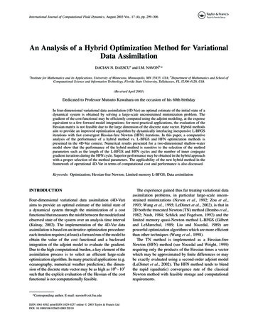
upper band is the period where only the financial instrument is held, and the zone below thelower band is where only cash is held, illustrated by Figure 3.Stock OnlySellSellPhase 3BuyPhase 2Phase 1BuyCash OnlyBuyFigure 3 Notation of Buy and Sell Signals on Bollinger BandsTimeSince the stock is bought as much as possible after the price movement exiting from the‘cash only’ zone, there is no extra buy signals when the trend enters the ‘stock only’ zone inthe first two buy-sell phases shown in Figure 3. After Phase 2, the price level does nottouch the lower band, which is supposed to trigger buy activities at relatively low price.Therefore, it is necessary to set remedial buy signal when the price trend enters the ‘stockonly’ zone again in Phase 3 to capture the profitable upward movement. In eachintersection, only one band is considered so no signal conflicts can occur.3.3. Asymmetric Bollinger BandsBullish and bearish trends may not perform in the same patterns in terms of return andvolatility, implying that the trend following strategies for upward and downward trendsmay be different. Bollinger Bands have the potential to address to this issue sinceindividual bands can provide responds to the changing trend separately. When there is astrong upward (downward) trend, the price is very likely to move to a relatively high (low)level, which is indicated by the breakout from the upper (lower) bound of Bollinger Bands.9