Transcription
The E ect of Television Advertising inUnited States ElectionsJohn Sides Lynn Vavreck†Christopher Warshaw‡August 24, 2021Conditionally accepted at the American Political Science ReviewAbstractWe provide a comprehensive assessment of the impact of television advertising onUnited States election outcomes from 2000-2018. We expand on previous researchby including presidential, Senate, House, gubernatorial, Attorney General, and stateTreasurer elections and using both di erence-in-di erences and border-discontinuityresearch designs to help identify the causal e ect of advertising. We find that televisedbroadcast campaign advertising matters up and down the ballot, but it has muchlarger e ects in down-ballot elections than in presidential elections. Using survey andvoter registration data from multiple election cycles, we also show that the primarymechanism for ad e ects is persuasion, not the mobilization of partisans. Our resultshave implications for the study of campaigns and elections as well as voter decisionmaking and org/10.7910/DVN/F8JXHR. We wish to thank the editors and anonymous reviewers fortheir feedback. We are grateful for feedback from Justin de Benedictis-Kessner, David Broockman, KevinCollins, Rich Davis, James Mulhall, Robert Erikson, Anthony Fowler, Don Green, Andrew Hall, EthanPorter, Julian Wamble, Michael Miller, Eitan Hersh, Seth Hill, Dan Hopkins, Josh Kalla, Otis Reid, AaronStrauss, Travis Ridout, and Daron Shaw. We also appreciate feedback from participants in workshopsat George Washington University, Vanderbilt University, Stony Brook University, and the University ofMaryland. William R. Kenan, Jr.Professor, Department of Political Science, Vanderbilt University,john.m.sides@vanderbilt.edu†Marvin Ho enberg Professor of American Politics, Department of Political Science, UCLAlvavreck@ucla.edu, ORCID: https://orcid.org/0000-0003-4582-7960‡Associate Professor, Department of Political Science, George Washington University, warshaw@gwu.edu,ORCID: https://orcid.org/0000-0002-2769-40281
How much does televised campaign advertising a ect election outcomes in the UnitedStates? This has been a pertinent question since the first televised advertisements were airedduring a 1950 Connecticut Senate election and then by President Dwight Eisenhower’s 1952campaign (Benoit 2018). Answering this question helps illuminate the motivations behindvoting behavior, the influence of mass communication on the electorate, and how muchcandidates’ resources and messages can help them win elections. Moreover, the aggregatee ect of televised advertising may determine the actual winner in at least some races, therebya ecting the composition of government and the direction of public policy.Political campaigns spend a great deal of money on television advertising. According toFowler, Ridout, and Franz (2016), over 2.75 billion was spent to air over 4.25 million ads inthe 2015-2016 election cycle. This includes about 1 million airings in the presidential race,1 million airings in Senate races, 620,000 airings in House races, and 1.25 million airings inother races at the state and local levels. Spending on television advertising constitutes about45 percent of a typical congressional campaign’s budget (Jacobson and Carson 2019).Research on televised political advertising has made significant progress in estimating itsimpact on voting behavior (for overviews, see Goldstein and Ridout 2004; Fowler, Franz,and Rideout 2016; Jacobson 2015). Studies have found associations between television advertising and individual vote intentions, aggregate vote shares, or both (e.g., Huber andArceneaux 2007; Ridout and Franz 2011; Sides and Vavreck 2013; Spenkuch and Toniatti2018). In presidential general elections, the persuasive impact of television advertising appears to be larger than the impact of other electioneering, such as canvassing or mail, whoseimpact is quite small, even zero (Kalla and Broockman 2018).But there are significant limitations to what we know about the e ects of televised campaign advertising on election outcomes. Most importantly, the extant literature is almostentirely focused on presidential general elections (e.g., Johnston, Hagen, and Jamieson 2004;Gordon and Hartmann 2013; Shaw 2006; Sides and Vavreck 2013; Sides, Tesler, and Vavreck2018; Spenkuch and Toniatti 2018). Only a few studies have examined advertising e ects1
in Senate elections (Jacobson 1975; Goldstein and Freedman 2000; Ridout and Franz 2011;Fowler, Ridout, and Franz 2016; Wang, Lewis, and Schweidel 2018) or House elections (Jacobson 1975; Hill et al. 2013).1 Just two studies have examined gubernatorial elections andboth focus on survey-based vote intentions rather than election results (Hill et al. 2013;Gerber et al. 2011). To our knowledge, there has been no published research on the e ectof advertising in down-ballot state-level races, such as elections for state Attorney General.And, most importantly, no study has used a comparable, credible research design to studyadvertising e ects across multiple levels of office. The most relevant prior studies comparepresidential and Senate elections (Jacobson 1975; Ridout and Franz 2011; Fowler, Ridout,and Franz 2016) and find that advertising in Senate elections appears to have larger e ectson election outcomes than does advertising in presidential elections. This paucity of studiesillustrates the conclusion of Kalla and Broockman (2018), who, after canvassing the available experiments on persuasion in general election campaigns, argue that “more evidence”on televised advertising “would clearly be welcome” (163). We aim to provide that evidence.Campaign advertisements provide information to voters that may change the balanceof considerations they hold about candidates in a given contest. As the balance shifts,citizens may change their views of the candidates (persuasion) or change their mind aboutwhether to vote at all (mobilization). If advertising a ects election outcomes mainly throughpersuasion at the individual level, it should have larger e ects in down-ballot races than inpresidential races. This is because voters know less and have weaker opinions about downballot candidates relative to presidential candidates. But if advertising works mainly throughmobilization, potentially altering the partisan composition of the electorate, voters’ decisionsto stay home or turn out should a ect all races on the ballot similarly. If so, there should1. Scholars have investigated the tone of campaigning in Senate elections and its possible e ects on electionoutcomes (Lau and Pomper 2004) and how voter decision-making depends on the “intensity of Senatecampaigns” (Kahn and Kenney 1999; Westlye 1991), which are related to but distinct from our focus. Studiesof U.S. House elections focus mainly on candidate spending as a proxy for specific forms of campaigningsuch as advertising (e.g., Jacobson 1978; Green and Krasno 1988). Only occasionally have scholars tried toisolate the e ects of House electioneering activities (Jacobson 1975; Ansolabehere and Gerber 1994; Schuster2020).2
be little heterogeneity across offices in the e ect of ads on election outcomes.We test these expectations by examining the impact of broadcast television advertising onelection outcomes in the 5 presidential elections from 2000–2018 and also in 331 U.S. Senateelections, 226 gubernatorial elections, 3,859 U.S. House elections, and 237 other state-levelelections during this time period. In total, we examine over 4,500 di erent races. To addressthe possibility that campaigns may place ads in media markets where they expect to dowell (Erikson and Tedin 2019, 250), we employ research designs that strengthen the causalinterpretation of our findings, including time-series cross-sectional models with a di erencein-di erences design (Angrist and Pischke 2009) and a border-discontinuity design (Spenkuchand Toniatti 2018).We find that the e ect of ad airings is much larger in down-ballot elections than inpresidential elections. The apparent e ect of an individual airing is two to four times largerin gubernatorial, U.S. House, and U.S. Senate elections and ten to nineteen times larger inother statewide races, compared to presidential elections.We also provide evidence that persuasion is the primary mechanism through which thesedi ering e ects of advertising emerge. Drawing on surveys of hundreds of thousands ofvoters across eight election cycles, we show that voters have less information and weakeropinions about the candidates in down-ballot races compared to presidential candidates andthat in these down-ballot races television advertising is more strongly associated with voters’knowledge of the candidates, evaluations of the candidates, and ideological congruence withthe candidates than it is in presidential races. By contrast, we find less evidence for anotherpossible mechanism: that television advertising a ects election outcomes by changing thepartisan composition of the electorate. Drawing on administrative data from six di erentelection cycles, we show that advertising is not consistently associated with the relativeturnout of Democrats and Republicans. Moreover, we find that ads for one race do notsubstantially “spill over” and a ect outcomes at another level of office, as would be true ifadvertising altered the partisan composition of the voters in any election year.3
Our paper has several key implications for the study of voting behavior and elections.Despite increasing partisan loyalty among American voters, some voters still respond totelevision advertising. This is particularly true in down-ballot elections. Indeed, whiletelevision advertising is likely to swing only very close presidential elections, infusions oftelevision advertising could swing a larger number of close down-ballot elections. Thus,the e ort that candidates, political parties, and outside groups invest in raising money for,producing, and airing television advertising pays dividends. Mass communication in electoralcampaigns matters, even in a more polarized electorate.1Theoretical MotivationDoes television advertising in U.S. elections a ect election outcomes? And should its e ectvary across levels of office? Drawing on literatures in psychology, political science, economics,and political communication, we assemble a set of expectations for both questions.Campaign advertising can persuade voters if it provides novel information that a ectstheir attitudes about one or both candidates. Prior research on attitude change shows thatpeople can be susceptible to persuasion, but that there are many obstacles to changing someone’s mind (e.g., DellaVigna and Gentzkow 2010; Petty, Priester, and Wegener 2014; Searsand Kosterman 1994). This well-established idea is central to theories of information processing in political science. For one, Zaller (1992) argues that attitude change in response toinformation is conditional on partisanship and other predispositions (“partisan resistance”)as well as the number of existing considerations that someone has about an attitude object(“inertial resistance”). For another, Lodge and Taber (2013) argue that once people thinkabout a political object, that object has an “a ective tag” (a positive or negative feeling)stored in memory, which then influences subsequent information-processing and leads to“motivated reasoning.” Both accounts suggest that persuasion is possible, but when peoplehave relevant prior attitudes, and especially strongly held attitudes, they are less likely to4
change their attitudes in response to new information.This pattern suggests more potential for persuasion in down-ballot races, where peoplehave thought less about the candidates and have fewer stored considerations and weakera ective tags, if any. As Delli Carpini and Keeter (1996) show, Americans are more familiarwith national political figures, such as the president and vice-president, than with figureslike U.S. Senator. Indeed, the percentage of Americans who could name both Senatorsdeclined between 1947 and 1989, even as the percentage who could name the vice-presidentincreased. Likewise, Hopkins (2018) shows that the percentage of Americans who can nametheir governor declined from 87% in 1947 to 66% in 2007. Hopkins also finds that Americanscould supply less information about governors than presidents when asked to describe them,and were less likely to search the Internet for information about governors than presidents.These declines are likely linked to the decreasing amount of news coverage of state andlocal politics (Hayes and Lawless, Forthcoming). Research on congressional elections alsofinds di erences in knowledge across levels of office. In particular,a a larger percentage ofAmericans can recall and recognize the names of U.S. Senate candidates than U.S. Housecandidates (Jacobson and Carson 2019). Here again, knowledge of congressional candidatesis linked to how much local news covers congressional campaigns (Hayes and Lawless 2018).These informational and attitudinal asymmetries across levels of political office imply thatnew information—such as in television advertising—should more strongly influence views ofdown-ballot candidates than views of presidential candidates.2 The persuasive potential ofcampaigns and campaign advertising is evident in previous research. Campaigns provide information to voters, who become better able to name candidates (Elms and Sniderman 2006;Jacobson 2006) and identify where the candidates stand on political issues (Patterson andMcClure 1972; Franklin 1991; Alvarez 1998; Johnston, Hagen, and Jamieson 2004). Television advertising specifically contributes both to informational gains (Freedman, Franz, andGoldstein 2004) and changes in attitudes toward the candidates (Freedman and Goldstein2. Even in presidential races, advertising may have a larger e ect on views of the lesser-known candidate(Broockman and Kalla 2020).5
1999; Johnston, Hagen, and Jamieson 2004; Huber and Arceneaux 2007; Ridout and Franz2011; Coppock, Hill, and Vavreck 2020).3 Moreover, Huber and Arceneaux (2007) show thatchanges in attitudes toward the candidates—i.e., persuasion—are an important mechanismby which television advertisements influence vote intentions. This potential for persuasionis in line with the strategies of candidates themselves, who air advertising primarily onprograms with audiences containing many swing voters (Lovett and Peress 2010).Synthesizing this prior work on information, persuasion, and advertising leads to severalexpectations. We expect that television advertising has a larger impact on election outcomesin down-ballot races for Congress, governor, and other statewide offices than in presidentialraces. In terms of pathways for this e ect, we expect that voters are less likely to haveopinions about down-ballot candidates and, when they do have opinions, they are weakerthan their opinions about presidential candidates. Therefore, we expect that television advertising has a larger e ect on voters’ knowledge and attitudes about down-ballot candidatescompared to presidential candidates. Evidence for these latter two expectations will suggestthat persuasion is a key mechanism by which advertising a ects election outcomes.A contrasting expectation is that television advertising a ects outcomes mainly throughits e ect on whether partisans turn out to vote. Although political advertising does notappear to have a significant e ect on overall turnout (Ashworth and Clinton 2007; Krasnoand Green 2008; Spenkuch and Toniatti 2018; Lovett and Peress 2010), it could a ect thepartisan composition of the electorate if candidates’ ads mobilize their own partisans andde-mobilize their opponent’s partisans in roughly equal amounts. Prior research has foundthat the partisan composition of the electorate is associated with partisan campaign activityaggregated across levels of office (McGhee and Sides 2005) as well as national party spending(Holbrook and McClurg 2011). Most relevant to this study is Spenkuch and Toniatti (2018),who find that presidential television advertising is associated with the partisan compositionof the electorate in the 2004-12 elections.3. Beyond the direct e ects of ads, they may also help inform voters by spurring people to seek informationvia other sources (Canen and Martin 2020).6
If advertising matters mainly through partisan mobilization, then, contrary to the firstexpectation, advertising should have a similar relationship to election outcomes across levelsof office. Assuming that partisans vote for their party’s candidate at similar rates acrosslevels of office, any shifts in partisan turnout induced by advertising should a ect candidatesup and down the ballot in roughly equal amounts. We test for partisan mobilization in twoways: by examining the relationship between advertising and partisan turnout across severalelection cycles and by examining the relationship between advertising at one level of officeand outcomes at other levels. Any “spillover” across levels of office suggests that ads a ectpartisan turnout and thus a ect races other than the one the ads are targeting.2Data and Research DesignTo evaluate the e ect of political advertising, we built a panel dataset of election returnsand advertising data at the county level that substantially extends similar datasets in otherwork (e.g., Shaw 2006; Ridout and Franz 2011; Sides and Vavreck 2013; Fowler, Ridout,and Franz 2016; Sides, Tesler, and Vavreck 2018). This dataset’s considerable temporal andgeographic scope, alongside a credible research design, provides a rigorous test of the causale ect of advertising on thousands of election outcomes.We assembled 2000-2018 national, state, and local election returns from various sources.For presidential, senate, and gubernatorial elections, we used data from CQ’s Voting andElections Collection. For House elections during this period, we used data from the Atlas ofU.S. Elections (Leip 2016), which break the congressional election returns down by county.4For other state offices (i.e., attorney general and treasurer), we used crowd-sourced countylevel data from OurCampaigns.com.5Our primary treatment variable is the net Democratic advantage in the number of broadcast television ad airings in a county over the last two months (64 days) of the campaign.4. Both the CQ and Atlas of U.S. Elections data were obtained under a restricted license.5. Thirty-six states elect state treasurers and 43 elect attorneys general.7
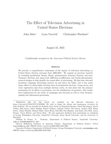
Similar measures have been used in prior research on advertising e ects (e.g., Franz and Ridout 2007; Spenkuch and Toniatti 2018; Lovett and Peress 2010). To be sure, this measuredoes not capture all advertising, an increasing percentage of which is aired on local cableoutlets or online. But broadcast television advertisements constituted the vast majority ofcampaign advertising during this time period (Fowler, Ridout, and Franz 2016).We calculate the net Democratic advertising advantage by taking the di erence betweenthe number of Democratic and Republican ad airings for a particular race in each mediamarket using advertising data obtained under license from the Wesleyan Media Project andthe Wisconsin Advertising Project (Fowler, Franz, and Ridout 2020).6 These data includethe top 75 media markets in the 2000 election cycle, the top 100 markets in the 2002,2004, and 2006, cycles, and all 210 media markets since 2008.7 Figure 1 displays the netDemocratic ad advantage in each media market for an illustrative set of offices and years. Itshows not only the comprehensiveness of our data but how much advertising volume variesacross offices and geography.We include all general election advertising supporting the Democratic and Republicancandidates in each race, including ads aired by the candidate’s campaign, parties, and outsidegroups.8 Our focus on advertising in the last two months of the campaign reflects the extantfinding that ads aired closer to Election Day are more e ective than ads aired earlier in theelection cycle (e.g., Sides and Vavreck 2013; Sides, Tesler, and Vavreck 2018).9One limitation of this measure is that it does not account for the size of the television6. The Wisconsin Ads Project data can be obtained at roject/ and the Wesleyan Media Project can be obtained at https://mediaproject.wesleyan.edu/dataaccess/.7. We assign counties to media markets based on the Nielsen definitions of media markets. We use dataon these assignments from Sood (2016) and manually checked how these assignments vary over time basedon individual Broadcasting and Cable Yearbooks.8. The Wesleyan Media Project and Wisconsin Advertising Project data include a variable that identifiesprimary and general elections ads in 2000 and 2012-2020. We used this variable to drop primary electionads from our analysis in those years. In other years (2002-2010) we dropped all ads that were aired beforethe primary election date in each state.9. In Appendix G, we provide more evidence, showing that ads aired in the summer have no e ect onelection outcomes, but ads aired in September and in October both a ect outcomes and to roughly the sameextent.8
Dem. Ad. Advantage 20020Dem. Ad. Advantage40(a) Presidential Race, 2012Dem. Ad. Advantage 40 200 2002040(b) Senate Races, 2012Dem. Ad. Advantage20(c) Governor Races, 2014 1001020(d) House Races, 2012Figure 1: Democratic Advertising Advantage (in 100s of ads) across Geography in an Illustrative Set of Offices and Years. Positive (bluer) values show a pro-Democratic advantageand negative (redder) values show a pro-Republican advantage.audience that could have seen each ad airing. However, counts of ad airings are highlycorrelated with measures, such as gross ratings points, that do attempt to account for thenumber of people possibly exposed.10 For instance, the correlation between airings andGRP’s at the candidate-market-day level was .99 in the 2012 presidential race.We use two parallel research designs to estimate the causal e ect of television advertisingon election outcomes. The first design includes all U.S. counties in the media markets10. In 2006, we have measures of both ad airings and gross ratings points (GRP’s) for 69 candidates in9 media markets across 5 states (MI, MN, OH, IL, IN). These candidates were running for U.S. House ofRepresentatives (60), Senate (4), and Governor (5). Across the 42 days leading up to election day, thecorrelation at the candidate-market-day level between ad airings and GRP’s ranges from .89 to 1.0 forcandidates who ran ten or more ads. The average correlation across all candidate-market-days is .97. In2012, the correlation between ads aired and GRP’s for presidential candidates Barack Obama and MittRomney was similarly high. In the 159 days leading up to the 2012 general election, the correlation betweenairings and GRP’s at the candidate-market-day level was .99 for both Obama and Romney. We estimatethat each ad airing was worth 3-4 GRP’s in the 2012 presidential race.9
contained in the advertising data (e.g., all counties starting in 2008 and a subset of countiesbefore that). We include either county fixed e ects to account for time-invariant confoundersin each county or a lagged outcome variable in lieu of county fixed e ects.11 These accountfor the overall partisan orientation of each county. We also include state-year fixed e ects tocontrol for time-varying confounders at the state and national levels (Fowler and Hall 2018;de Benedictis-Kessner and Warshaw 2020). The state-year fixed e ects account for trends inthe political preferences of each state across election years, such as the pro-Republican trendin Ohio or the pro-Democratic trend in Arizona. They also account for race-specific dynamicsin each state, such as the strength of the candidates and any incumbency advantage. In ouranalysis of congressional districts, we use district-year fixed e ects to account for the strengthof the candidates in each race. Thus, this research design isolates the e ects of advertisingfrom other aspects of candidates’ quality and spending.12Although this panel design addresses a host of possible confounders, it may miss the e ectof unobserved time-varying confounders at the media market or county levels that could biasour estimates. In particular, campaigns could be strategically targeting their spending inareas of a state where they expect to do well by using information, such as internal polls,that is unavailable to researchers.Our second research design accounts for this possibility by restricting the sample tocounties in the same state that are adjacent to one another but on di erent sides of theborder of a media market. Spenkuch and Toniatti (2018) use this design to study the e ects oftelevision advertising in the 2004-2012 presidential elections. Similarly, Huber and Arceneaux(2007) use media market boundaries to study the e ects of television advertising in the 200011. We do not include county fixed e ects in the model with the lagged outcome variable to avoid issuesof Nickell bias that can arise in datasets with a small number of time periods (Nickell 1981; Beck and Katz2011).12. We cluster our standard errors at the county level to account for serial correlation in errors. Wealso cluster by media market-year to account for the fact that each county in a market receives the samedosage of advertising during a particular election year (Abadie et al. 2017). In Appendix A, we show howthe standard errors for our point estimates of advertising e ects in presidential races vary using di erentclustering strategies. In general, di erent clustering strategies produce similar standard errors and muchsmaller standard errors than if we did not cluster at all.10
presidential election. Other studies have used discontinuities in treatment exposure acrosscounty or state boundaries to study the incumbency advantage (Ansolabehere, Snowberg,and Snyder 2006) and the e ects of policies like Medicare expansion and right-to-work laws(e.g., Clinton and Sances 2018; Feigenbaum, Hertel-Fernandez, and Williamson 2018).The intuition behind the border county design is that within a state, adjacent countiesthat straddle the border of a media market are likely to be similar to one another exceptthat they are on di erent sides of the media market boundary and therefore may be exposedto di erent levels of television advertising. Moreover, this variation in advertising spendingis plausibly exogenous to characteristics of these border counties. It seems unlikely thatadvertising is targeted based on the characteristics of specific border counties, especiallybecause the counties on media market boundaries exclude the urban cores of most mediamarkets. Only about 5% of the nation’s population lives in a county on a within-state mediamarket boundary (Spenkuch and Toniatti 2018). For evidence that border county designsachieve balance on many characteristics of counties that could also a ect election outcomes,see Spenkuch and Toniatti (2018).To illustrate this design, Figure 2 shows the border counties in Pennsylvania (shaded ingrey). It confirms that most major cities (e.g., Philadelphia, Pittsburgh, Erie, and Scranton)are not in border counties. The adjacent counties that do lie along media market borderstend to be similar to one another. For example, Indiana and Cambria counties are adjacentto each other along the boundary between the Pittsburgh and Johnstown-Altoona mediamarkets. Both counties are largely rural areas where Mitt Romney received about 58% ofthe vote in the 2012 presidential election.To execute the border county design, we match each county in a state with every otheradjacent county that lies on the other side of a media market boundary. The unit of analysisbecomes the border county pair, with the two counties on opposite sides of a media marketboundary. Thus, a particular county could be in this sample multiple times if it bordersmultiple counties in this fashion. For this reason, the overall sample size is larger in this11
Figure 2: Illustration of the Border Counties Design in Pennsylvania. The dark lines indicatemedia market boundaries. The shaded counties, which lie along a media market boundarynext to another county in Pennsylvania, are the ones included in the border county stownDMANew YorkDMAWilkes ington DCDMAHarrisburgDMAdesign than the first design.13 In analyzing this sample of border counties, we includecounty fixed e ects to account for time-invariant confounders in each county. Crucially, wealso include year-specific fixed e ects for each pair of border counties. This accounts for thee ect of any year-specific unobserved confounders in each border-pair of counties, such astrends in their partisanship or ideology. Thus, only confounders that vary between bordercounties within a particular election cycle could bias our results using this design. Whileit is impossible to rule out these confounders, there appears to be no correlation betweenchanges in political advertising and border counties’ time-varying observable characteristics(Spenkuch and Toniatti 2018).13. We cluster standard errors in the border county sample by county and media market border-year toensure that this process does not artificially increase our statistical precision (Abadie et al. 2017).12
To test the assumption that there are no time-varying confounders, typically called theparallel trends assumption, we examined whether future values of television advertising appear to have a significant e ect on current outcomes. F
We test these expectations by examining the impact of broadcast television advertising on election outcomes in the 5 presidential elections from 2000-2018 and also in 331 U.S. Senate elections, 226 gubernatorial elections, 3,859 U.S. House elections, and 237 other state-level