Transcription
RFoundations and Trends inTheoretical Computer ScienceVol. 8, Nos. 1–2 (2012) 1–141c 2013 N. K. Vishnoi DOI: 10.1561/0400000054Lx bLaplacian Solvers andTheir Algorithmic ApplicationsBy Nisheeth K. VishnoiContentsPreface2Notation6I8Basics1 Basic Linear Algebra1.11.2Spectral Decomposition of Symmetric MatricesMin–Max Characterizations of Eigenvalues99122 The Graph Laplacian142.12.21416The Graph Laplacian and Its EigenvaluesThe Second Eigenvalue and Connectivity3 Laplacian Systems and Solvers183.13.23.33.418191920System of Linear EquationsLaplacian SystemsAn Approximate, Linear-Time Laplacian SolverLinearity of the Laplacian Solver
4 Graphs as Electrical Networks224.14.24.34.4Incidence Matrices and Electrical NetworksEffective Resistance and the Π MatrixElectrical Flows and EnergyWeighted Graphs22242527IIApplications285 Graph Partitioning I The Normalized Laplacian295.15.25.3293134Graph ConductanceA Mathematical ProgramThe Normalized Laplacian and Its Second Eigenvalue6 Graph Partitioning IIA Spectral Algorithm for Conductance6.16.2Sparse Cuts from 1 EmbeddingsAn 1 Embedding from an 22 Embedding3737407 Graph Partitioning III Balanced Cuts447.17.2The Balanced Edge-Separator ProblemThe Algorithm and Its Analysis44468 Graph Partitioning IVComputing the Second Eigenvector498.18.24950The Power MethodThe Second Eigenvector via Powering9 The Matrix Exponential and Random Walks549.19.29.3545659The Matrix ExponentialRational Approximations to the ExponentialSimulating Continuous-Time Random Walks
10 Graph Sparsification ISparsification via Effective Resistances6210.1 Graph Sparsification10.2 Spectral Sparsification Using Effective Resistances10.3 Crude Spectral Sparsfication62646711 Graph Sparsification IIComputing Electrical Quantities6911.1 Computing Voltages and Currents11.2 Computing Effective Resistances697112 Cuts and Flows7512.112.212.312.4Maximum Flows, Minimum CutsCombinatorial versus Electrical Flowss, t-MaxFlows, t-Min Cut75777883IIITools8613 Cholesky Decomposition Based Linear Solvers8713.1 Cholesky Decomposition13.2 Fast Solvers for Tree Systems878914 Iterative Linear Solvers IThe Kaczmarz Method9214.1 A Randomized Kaczmarz Method14.2 Convergence in Terms of Average Condition Number14.3 Toward an Õ(m)-Time Laplacian Solver92949615 Iterative Linear Solvers IIThe Gradient Method99
15.1 Optimization View of Equation Solving15.2 The Gradient Descent-Based Solver9910016 Iterative Linear Solvers IIIThe Conjugate Gradient Method10316.116.216.316.4Krylov Subspace and A-OrthonormalityComputing the A-Orthonormal BasisAnalysis via Polynomial MinimizationChebyshev Polynomials — Why ConjugateGradient Works16.5 The Chebyshev Iteration16.6 Matrices with Clustered Eigenvalues10310510717 Preconditioning for Laplacian Systems11417.1 Preconditioning17.2 Combinatorial Preconditioning via Trees17.3 An Õ(m4/3 )-Time Laplacian Solver11411611718 Solving a Laplacian System in Õ(m) Time11918.1 Main Result and Overview18.2 Eliminating Degree 1, 2 Vertices18.3 Crude Sparsification Using Low-StretchSpanning Trees18.4 Recursive Preconditioning — Proof of theMain Theorem18.5 Error Analysis and Linearity of the Inverse11912219 Beyond Ax b The Lanczos Method12919.1 From Scalars to Matrices19.2 Working with Krylov Subspace19.3 Computing a Basis for the Krylov Subspace129130132References136110111112123125127
RFoundations and Trends inTheoretical Computer ScienceVol. 8, Nos. 1–2 (2012) 1–141c 2013 N. K. Vishnoi DOI: 10.1561/0400000054Lx bLaplacian Solvers andTheir Algorithmic ApplicationsNisheeth K. VishnoiMicrosoft Research, India, nisheeth.vishnoi@gmail.comAbstractThe ability to solve a system of linear equations lies at the heart of areassuch as optimization, scientific computing, and computer science, andhas traditionally been a central topic of research in the area of numerical linear algebra. An important class of instances that arise in practice has the form Lx b, where L is the Laplacian of an undirectedgraph. After decades of sustained research and combining tools fromdisparate areas, we now have Laplacian solvers that run in time nearlylinear in the sparsity (that is, the number of edges in the associatedgraph) of the system, which is a distant goal for general systems. Surprisingly, and perhaps not the original motivation behind this line ofresearch, Laplacian solvers are impacting the theory of fast algorithmsfor fundamental graph problems. In this monograph, the emergingparadigm of employing Laplacian solvers to design novel fast algorithmsfor graph problems is illustrated through a small but carefully chosenset of examples. A part of this monograph is also dedicated to developing the ideas that go into the construction of near-linear-time Laplaciansolvers. An understanding of these methods, which marry techniquesfrom linear algebra and graph theory, will not only enrich the tool-setof an algorithm designer but will also provide the ability to adapt thesemethods to design fast algorithms for other fundamental problems.
PrefaceThe ability to solve a system of linear equations lies at the heart of areassuch as optimization, scientific computing, and computer science and,traditionally, has been a central topic of research in numerical linearalgebra. Consider a system Ax b with n equations in n variables.Broadly, solvers for such a system of equations fall into two categories.The first is Gaussian elimination-based methods which, essentially, canbe made to run in the time it takes to multiply two n n matrices,(currently O(n2.3. ) time). The second consists of iterative methods,such as the conjugate gradient method. These reduce the problemto computing n matrix–vector products, and thus make the runningtime proportional to mn where m is the number of nonzero entries, orsparsity, of A.1 While this bound of n in the number of iterations istight in the worst case, it can often be improved if A has additionalstructure, thus, making iterative methods popular in practice.An important class of such instances has the form Lx b, where Lis the Laplacian of an undirected graph G with n vertices and m edges1 Strictlyspeaking, this bound on the running time assumes that the numbers have boundedprecision.2
Preface3with m (typically) much smaller than n2 . Perhaps the simplest settingin which such Laplacian systems arise is when one tries to compute currents and voltages in a resistive electrical network. Laplacian systemsare also important in practice, e.g., in areas such as scientific computingand computer vision. The fact that the system of equations comes froman underlying undirected graph made the problem of designing solversespecially attractive to theoretical computer scientists who entered thefray with tools developed in the context of graph algorithms and withthe goal of bringing the running time down to O(m). This effort gainedserious momentum in the last 15 years, perhaps in light of an explosivegrowth in instance sizes which means an algorithm that does not scalenear-linearly is likely to be impractical.After decades of sustained research, we now have a solver for Laplacian systems that runs in O(m log n) time. While many researchers havecontributed to this line of work, Spielman and Teng spearheaded thisendeavor and were the first to bring the running time down to Õ(m)by combining tools from graph partitioning, random walks, and lowstretch spanning trees with numerical methods based on Gaussian elimination and the conjugate gradient. Surprisingly, and not the originalmotivation behind this line of research, Laplacian solvers are impactingthe theory of fast algorithms for fundamental graph problems; givingback to an area that empowered this work in the first place.That is the story this monograph aims to tell in a comprehensivemanner to researchers and aspiring students who work in algorithmsor numerical linear algebra. The emerging paradigm of employingLaplacian solvers to design novel fast algorithms for graph problemsis illustrated through a small but carefully chosen set of problemssuch as graph partitioning, computing the matrix exponential, simulating random walks, graph sparsification, and single-commodity flows. Asignificant part of this monograph is also dedicated to developing thealgorithms and ideas that go into the proof of the Spielman–Teng Laplacian solver. It is a belief of the author that an understanding of thesemethods, which marry techniques from linear algebra and graph theory,will not only enrich the tool-set of an algorithm designer, but will alsoprovide the ability to adapt these methods to design fast algorithmsfor other fundamental problems.
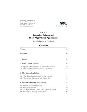
4PrefaceHow to use this monograph. This monograph can be used as thetext for a graduate-level course or act as a supplement to a course onspectral graph theory or algorithms. The writing style, which deliberately emphasizes the presentation of key ideas over rigor, should evenbe accessible to advanced undergraduates. If one desires to teach acourse based on this monograph, then the best order is to go throughthe sections linearly. Essential are Sections 1 and 2 that contain thebasic linear algebra material necessary to follow this monograph andSection 3 which contains the statement and a discussion of the maintheorem regarding Laplacian solvers. Parts of this monograph can alsobe read independently. For instance, Sections 5–7 contain the Cheegerinequality based spectral algorithm for graph partitioning. Sections 15and 16 can be read in isolation to understand the conjugate gradientmethod. Section 19 looks ahead into computing more general functionsthan the inverse and presents the Lanczos method. A dependency diagram between sections appears in Figure 1. For someone solely interested in a near-linear-time algorithm for solving Laplacian systems, thequick path to Section 14, where the approach of a short and new proofis presented, should suffice. However, the author recommends going all1,2,358461011913151216147171918Fig. 1 The dependency diagram among the sections in this monograph. A dotted line fromi to j means that the results of Section j use some results of Section i in a black-box mannerand a full understanding is not required.
Preface5the way to Section 18 where multiple techniques developed earlier inthe monograph come together to give an Õ(m) Laplacian solver.Acknowledgments. This monograph is partly based on lecturesdelivered by the author in a course at the Indian Institute of Science, Bangalore. Thanks to the scribes: Deeparnab Chakrabarty,Avishek Chatterjee, Jugal Garg, T. S. Jayaram, Swaprava Nath, andDeepak R. Special thanks to Elisa Celis, Deeparnab Chakrabarty,Lorenzo Orecchia, Nikhil Srivastava, and Sushant Sachdeva for reading through various parts of this monograph and providing valuablefeedback. Finally, thanks to the reviewer(s) for several insightful comments which helped improve the presentation of the material in thismonograph.Bangalore15 January 2013Nisheeth K. VishnoiMicrosoft Research India
Notation The set of real numbers is denoted by R, and R 0 denotesthe set of nonnegative reals. We only consider real numbersin this monograph. The set of integers is denoted by Z, and Z 0 denotes the setof nonnegative integers. Vectors are denoted by boldface, e.g., u, v. A vector v Rnis a column vector but often written as v (v1 , . . . , vn ). Thetranspose of a vector v is denoted by v . For vectors u, v, their inner product is denoted by u, v oru v. For a vector v, v denotes its 2 or Euclidean norm wheredef v v, v . We sometimes also refer to the 1 or Mandef hattan distance norm v 1 ni 1 vi . The outer product of a vector v with itself is denoted byvv . Matrices are denoted by capitals, e.g., A, L. The transposeof A is denoted by A . We use tA to denote the time it takes to multiply the matrixA with a vector.6
Notation The A-norm of a vector v is denoted by v A def v Av. For a real symmetric matrix A, its real eigenvaluesdefare ordered λ1 (A) λ2 (A) · · · λn (A). We let Λ(A) [λ1 (A), λn (A)]. A positive-semidefinite (PSD) matrix is denoted by A 0and a positive-definite matrix A 0. The norm of a symmetric matrix A is denoted by A def max{ λ1 (A) , λn (A) }. For a symmetric PSD matrix A, A λn (A). Thinking of a matrix A as a linear operator, we denote theimage of A by Im(A) and the rank of A by rank(A). A graph G has a vertex set V and an edge set E. All graphsare assumed to be undirected unless stated otherwise. If thegraph is weighted, there is a weight function w : E R 0 .Typically, n is reserved for the number of vertices V , andm for the number of edges E . EF [·] denotes the expectation and PF [·] denotes the probability over a distribution F. The subscript is dropped whenclear from context. The following acronyms are used liberally, with respect to(w.r.t.), without loss of generality (w.l.o.g.), with high probability (w.h.p.), if and only if (iff), right-hand side (r.h.s.),left-hand side (l.h.s.), and such that (s.t.). Standard big-o notation is used to describe the limitingbehavior of a function. Õ denotes potential logarithmicfactors which are ignored, i.e., f Õ(g) is equivalent tof O(g logk (g)) for some constant k.7
Part IBasics
1Basic Linear AlgebraThis section reviews basics from linear algebra, such as eigenvalues andeigenvectors, that are relevant to this monograph. The spectral theoremfor symmetric matrices and min–max characterizations of eigenvaluesare derived.1.1Spectral Decomposition of Symmetric MatricesOne way to think of an m n matrix A with real entries is as a linearoperator from Rn to Rm which maps a vector v Rn to Av Rm .Let dim(S) be dimension of S, i.e., the maximum number of linearlyindependent vectors in S. The rank of A is defined to be the dimensionof the image of this linear transformation. Formally, the image of Adefis defined to be Im(A) {u Rm : u Av for some v Rn }, and thedefrank is defined to be rank(A) dim(Im(A)) and is at most min{m, n}.We are primarily interested in the case when A is square, i.e., m n, and symmetric, i.e., A A. Of interest are vectors v such thatAv λv for some λ. Such a vector is called an eigenvector of A withrespect to (w.r.t.) the eigenvalue λ. It is a basic result in linear algebrathat every real matrix has n eigenvalues, though some of them could9
10Basic Linear Algebrabe complex. If A is symmetric, then one can show that the eigenvaluesare real. For a complex number z a ib with a, b R, its conjugateis defined as z̄ a ib. For a vector v, its conjugate transpose v isthe transpose of the vector whose entries are conjugates of those in v.Thus, v v v 2 .Lemma 1.1. If A is a real symmetric n n matrix, then all of itseigenvalues are real.Proof. Let λ be an eigenvalue of A, possibly complex, and v be thecorresponding eigenvector. Then, Av λv. Conjugating both sides weobtain that v A λv , where v is the conjugate transpose of v.Hence, v Av λv v, since A is symmetric. Thus, λ v 2 λ v 2which implies that λ λ. Thus, λ R.Let λ1 λ2 · · · λn be the n real eigenvalues, or the spectrum, of Awith corresponding eigenvectors u1 , . . . , un . For a symmetric matrix, itsnorm isdef A max{ λ1 (A) , λn (A) }.We now study eigenvectors that correspond to distinct eigenvalues.Lemma 1.2. Let λi and λj be two eigenvalues of a symmetric matrixA, and ui , uj be the corresponding eigenvectors. If λi λj , then ui , uj 0.Proof. Given Aui λi ui and Auj λj uj , we have the following sequence of equalities. Since A is symmetric, u i A ui A. Thus, ui Auj λi ui uj on the one hand, and ui Auj λj ui uj on the other. Therefore, λj u i uj λi ui uj . This implies that ui uj 0 sinceλi λj .Hence, the eigenvectors corresponding to different eigenvalues areorthogonal. Moreover, if ui and uj correspond to the same eigenvalue λ, and are linearly independent, then any linear combination
1.1 Spectral Decomposition of Symmetric Matrices11is also an eigenvector corresponding to the same eigenvalue. The maximal eigenspace of an eigenvalue is the space spanned by all eigenvectorscorresponding to that eigenvalue. Hence, the above lemma implies thatone can decompose Rn into maximal eigenspaces Ui , each of which corresponds to an eigenvalue of A, and the eigenspaces corresponding todistinct eigenvalues are orthogonal. Thus, if λ1 λ2 · · · λk are theset of distinct eigenvalues of a real symmetric matrix A, and Ui is theeigenspace associated with λi , then, from the discussion above,k dim(Ui ) n.i 1Hence, given that we can pick an orthonormal basis for each Ui , we mayassume that the eigenvectors of A form an orthonormal basis for Rn .Thus, we have the following spectral decomposition theorem.Theorem 1.3. Let λ1 · · · λn be the spectrum of A with corre sponding eigenvalues u1 , . . . , un . Then, A ni 1 λi ui u i .defProof. Let B n i 1 λi ui ui .Then,Buj n λi ui u i uji 1 λj uj Auj .The above is true for all j. Since uj s are orthonormal basis of Rn , wehave for all v Rn , Av Bv. This implies A B.Thus, when A is a real and symmetric matrix, Im(A) is spanned by theeigenvectors with nonzero eigenvalues. From a computational perspective, such a decomposition can be computed in time polynomial in thebits needed to represent the entries of A.11 Tobe very precise, one can only compute eigenvalues and eigenvectors to a high enoughprecision in polynomial time. We will ignore this distinction for this monograph as we donot need to know the exact values.
121.2Basic Linear AlgebraMin–Max Characterizations of EigenvaluesNow we present a variational characterization of eigenvalues which isvery useful.Lemma 1.4. If A is an n n real symmetric matrix, then the largesteigenvalue of A isλn (A) v Av.v Rn \{0} v vmaxProof. Let λ1 λ2 · · · λn be the eigenvalues of A, and letu1 , u2 , . . . , un be the corresponding orthonormal eigenvectors whichspan Rn . Hence, for all v Rn , there exist c1 , . . . , cn R such that v i ci ui . Thus, ci uici ui , v, v ii c2i .iMoreover,v Av ci uiλj uj uj ck uki j ci ck λj (u i uj ) · (uj uk )i,j,k i λnc2i λi c2i λn v, v .iHence, v 0,v Avv v λn . This implies,v Av λn .v Rn \{0} v vmaxk
1.2 Min–Max Characterizations of Eigenvalues13Now note that setting v un achieves this maximum. Hence, thelemma follows.If one inspects the proof above, one can deduce the following lemmajust as easily.Lemma 1.5. If A is an n n real symmetric matrix, then the smallesteigenvalue of A isλ1 (A) v Av.v Rn \{0} v vminMore generally, one can extend the proof of the lemma above to thefollowing. We leave it as a simple exercise.Theorem 1.6. If A is an n n real symmetric matrix, then for all1 k n, we haveλk (A) v Av,v Rn \{0},v ui 0, i {1,.,k 1} v vλk (A) v Av.v Rn \{0},v ui 0, i {k 1,.,n} v vminandmaxNotesSome good texts to review basic linear algebra are [35, 82, 85]. Theorem 1.6 is also called the Courant–Fischer–Weyl min–max principle.
2The Graph LaplacianThis section introduces the graph Laplacian and connects the secondeigenvalue to the connectivity of the graph.2.1The Graph Laplacian and Its EigenvaluesdefdefConsider an undirected graph G (V, E) with n V and m E .We assume that G is unweighted; this assumption is made to simplifythe presentation but the content of this section readily generalizes tothe weighted setting. Two basic matrices associated with G, indexedby its vertices, are its adjacency matrix A and its degree matrix D.Let di denote the degree of vertex i.defAi,j 1 if ij E,0 otherwise,anddefDi,j di0if i j,otherwise.defThe graph Laplacian of G is defined to be L D A. We often referto this as the Laplacian. In Section 5, we introduce the normalized14
2.1 The Graph Laplacian and Its Eigenvalues15Laplacian which is different from L. To investigate the spectral properties of L, it is useful to first define the n n matrices Le as follows: Fordefevery e ij E, let Le (i, j) Le (j, i) 1, let Le (i, i) Le (j, j) 1,/ {i, j}. The following then fol/ {i, j} or j and let Le (i , j ) 0, if i lows from the definition of the Laplacian and Le s.Lemma 2.1. Let L be the Laplacian of a graph G (V, E). Then, L e E Le .This can be used to show that the smallest eigenvalue of a Laplacianis always nonnegative. Such matrices are called positive semidefinite,and are defined as follows.Definition 2.1. A symmetric matrix A is called positive semidefinite(PSD) if λ1 (A) 0. A PSD matrix is denoted by A 0. Further, A issaid to be positive definite if λ1 (A) 0, denoted A 0.Note that the Laplacian is a PSD matrix.Lemma 2.2. Let L be the Laplacian of a graph G (V, E). Then,L 0.Proof. For any v (v1 , . . . , vn ),v Lv v Le ve E v Le ve E (vi vj )2e ij E 0.Hence, minv 0 v Lv 0. Thus, appealing to Theorem 1.6, we obtainthat L 0.
16The Graph LaplacianIs L 0? The answer to this is no: Let 1 denote the vector with allcoordinates 1. Then, it follows from Lemma 2.1 that L1 0 · 1. Hence,λ1 (L) 0.For weighted a graph G (V, E) with edge weights given by a weightfunction wG : E R 0 , one can definewG (ij) if ij E0otherwise,defAi,j anddefDi,j l wG (il)0if i jotherwise.Then, the definition of the Laplacian remains the same, namely, L D A.2.2The Second Eigenvalue and ConnectivityWhat about the second eigenvalue, λ2 (L), of the Laplacian? We willsee in later sections on graph partitioning that the second eigenvalueof the Laplacian is intimately related to the conductance of the graph,which is a way to measure how well connected the graph is. In thissection, we establish that λ2 (L) determines if G is connected or not.This is the first result where we make a formal connection between thespectrum of the Laplacian and a property of the graph.Theorem 2.3. Let L be the Laplacian of a graph G (V, E). Then,λ2 (L) 0 iff G is connected.Proof. If G is disconnected, then L has a block diagonal structure. Itsuffices to consider only two disconnected components. Assume the disconnected components of the graph are G1 and G2 , and the corresponding vertex sets are V1 and V2 . The Laplacian can then be rearrangedas follows: 0L(G1 ),L 0L(G2 )
2.2 The Second Eigenvalue and Connectivity17where L(Gi ) is a Vi Vi matrix for i 1, 2. Consider the vectordef 0 V1 , where 1 Vi and 0 Vi denote the all 1 and all 0 vectors ofx1 1 V2 dimension Vi , respectively. This is an eigenvector corresponding to thedef 1 V1 . Sincesmallest eigenvalue, which is zero. Now consider x2 0 V2 x2 , x1 0, the smallest eigenvalue, which is 0 has multiplicity at least2. Hence, λ2 (L) 0.For the other direction, assume that λ2 (L) 0 and that G is connected. Let u2 be the second eigenvector normalized to have length 1. 2Then, λ2 (L) u 2 Lu2 . Thus,e ij E (u2 (i) u2 (j)) 0. Hence, forall e ij E, u2 (i) u2 (j).Since G is connected, there is a path from vertex 1 to everyvertex j 1, and for each intermediate edge e ik, u2 (i) u2 (k).Hence, u2 (1) u2 (j), j. Hence, u2 (c, c, . . . , c). However, we alsoknow u2 , 1 0 which implies that c 0. This contradicts the factthat u2 is a nonzero eigenvector and establishes the theorem.NotesThere are several books on spectral graph theory which contain numerous properties of graphs, their Laplacians and their eigenvalues; see[23, 34, 88]. Due to the connection of the second eigenvalue of theLaplacian to the connectivity of the graph, it is sometimes called itsalgebraic connectivity or its Fiedler value, and is attributed to [28].
3Laplacian Systems and SolversThis section introduces Laplacian systems of linear equations and notesthe properties of the near-linear-time Laplacian solver relevant for theapplications presented in this monograph. Sections 5–12 cover severalapplications that reduce fundamental graph problems to solving a smallnumber of Laplacian systems.3.1System of Linear EquationsAn n n matrix A and vector b Rn together define a system of linearequations Ax b, where x (x1 , . . . , xn ) are variables. By definition,a solution to this linear system exists if and only if (iff) b lies in theimage of A. A is said to be invertible, i.e., a solution exists for all b, ifits image is Rn , the entire space. In this case, the inverse of A is denotedby A 1 . The inverse of the linear operator A, when b is restricted tothe image of A, is also well defined and is denoted by A . This is calledthe pseudo-inverse of A.18
3.2 Laplacian Systems3.219Laplacian SystemsNow consider the case when, in a system of equations Ax b, A Lis the graph Laplacian of an undirected graph. Note that this system is not invertible unless b Im(L). It follows from Theorem 2.3that for a connected graph, Im(L) consists of all vectors orthogonal tothe vector 1. Hence, we can solve the system of equations Lx b if b, 1 0. Such a system will be referred to as a Laplacian system oflinear equations or, in short, a Laplacian system. Hence, we can definethe pseudo-inverse of the Laplacian as the linear operator which takesa vector b orthogonal to 1 to its pre-image.3.3An Approximate, Linear-Time Laplacian SolverIn this section we summarize the near-linear algorithm known forsolving a Laplacian system Lx b. This result is the basis of the applications and a part of the latter half of this monograph is devoted to itsproof.Theorem 3.1. There is an algorithm LSolve which takes as inputa graph Laplacian L, a vector b, and an error parameter ε 0, andreturns x satisfying x L b L ε L b L ,def log 1/ε) time, wherewhere b L bT Lb. The algorithm runs in O(mm is the number of nonzero entries in L.Let us first relate the norm in the theorem above to the Euclideannorm. For two vectors v, w and a symmetric PSD matrix A,λ1 (A) v w 2 v w 2A (v w)T A(v w) λn (A) v w 2 .In other words, A /2 v w v w A A /2 v w .11Hence,the distortion in distances due to the A-norm is at most λn (A)/λ1 (A).
20Laplacian Systems and SolversFor the graph Laplacian of an unweighted and connected graph,when all vectors involved are orthogonal to 1, λ2 (L) replaces λ1 (L).It can be checked that when G is unweighted, λ2 (L) 1/poly(n) andλn (L) Tr(L) m n2 . When G is weighted the ratio between theL-norm and the Euclidean norm scales polynomially with the ratio ofthe largest to the smallest weight edge. Finally, note that for any twodefvectors, v w v w . Hence, by a choice of ε δ/poly(n) inTheorem 3.1, we ensure that the approximate vector output by LSolveis δ close in every coordinate to the actual vector. Note that since thedependence on the tolerance on the running time of Theorem 3.1 islogarithmic, the running time of LSolve remains Õ(m log 1/ε).3.4Linearity of the Laplacian SolverWhile the running time of LSolve is Õ(m log 1/ε), the algorithm produces an approximate solution that is off by a little from the exactsolution. This creates the problem of estimating the error accumulation as one iterates this solver. To get around this, we note an important feature of LSolve: On input L, b, and ε, it returns the vectorx Zb, where Z is an n n matrix and depends only on L and ε. Zis a symmetric linear operator satisfying(1 ε)Z L (1 ε)Z ,(3.1)and has the same image as L. Note that in applications, such as that inSection 9, for Z to satisfy Z L ε, the running time is increasedto Õ(m log(1/ελ2 (L))). Since in most of our applications λ2 (L) is at least1/poly(n), we ignore this distinction.NotesA good text to learn about matrices, their norms, and the inequalitiesthat relate them is [17]. The pseudo-inverse is sometimes also referred toas the Moore–Penrose pseudo-inverse. Laplacian systems arise in manyareas such as machine learning [15, 56, 89], computer vision [57, 73],partial differential equations and interior point methods [24, 30], andsolvers are naturally needed; see also surveys [75] and [84].
3.4 Linearity of the Laplacian Solver21We will see several applications that reduce fundamental graphproblems to solving a small number of Laplacian systems inSections 5–12. Sections 8 and 9 (a result of which is assumed inSections 5 and 6) require the Laplacian solver to be linear. The notableapplications we will not be covering are an algorithm to sample a random spanning tree [45] and computing multicommodity flows [46].Theorem 3.1 was first proved in [77] and the full proof appears in aseries of papers [78, 79, 80]. The original running time contained a verylarge power of the log n term (hidden in Õ(·)). This power has sincebeen reduced in a series of work [8, 9, 49, 62] and, finally, brought downto log n in [50]. We provide a proof of Theorem 3.1 in Section 18 alongwith its linearity property mentioned in this section. Recently, a simplerproof of Theorem 3.1 was presented in [47]. This proof does not requiremany of the ingredients such as spectral sparsifiers (Section 10), preconditioning (Section 17), and conjugate gradient (Section 16). Whilewe present a sketch of this proof in Section 14, we recommend that thereader go through the proof in Section 18 and, in the process, familiarize themselves with this wide array of techniques which may be usefulin general.
4Graphs as Electrical NetworksThis section introduces how a graph can be viewed as an electricalnetwork composed of resistors. It is shown how voltages and currentscan be computed by solving a Laplacian system. The notions of effective resistance, electrical flows, and their energy are presented. Viewinggraphs as electrical networks will play an important role in applicationspresented in Sections 10–12 and in the approach to a simple proof ofTheorem 3.1 presented in Section 14.4.1Incidence Matrices and Electrical NetworksGiven an undirected, unweighted graph G (V, E), consider an arbitrary orientation of its edges. Let B
Theoretical Computer Science Vol. 8, Nos. 1-2 (2012) 1-141 c 2013 N. K. Vishnoi DOI: 10.1561/0400000054 Lx b Laplacian Solvers and Their Algorithmic Applications By Nisheeth K. Vishnoi Contents Preface 2 Notation 6 I Basics 8 1 Basic Linear Algebra 9 1.1 Spectral Decomposition of Symmetric Matrices 9 1.2 Min-Max Characterizations of .