Transcription
Lecture 6: Option Pricing Using a One-stepBinomial TreeFriday, September 14, 12
An over-simplified model with surprisingly generalextensions a single time step from 0 to T two types of traded securities: stock S and a bond (or a money market account) current state: S(0) and the interest rate r (or the bond yield) are known only two possible states at T we want to price a call option in this over-simplified model what’s known and what’s not known: for each possible state, the stock price for this state is known, so is the option payoff we do not know which state we will end up with, just the belief that both have positiveprobabilities our goal: the price of the call option at time 0!Friday, September 14, 12
Why binomial model? surprisingly general after extensions more states can be included with multiple steps easy to program can handle any payoff functions (call, put, digital, etc.) even American options can be easily incorporated still in wide use in practice!Friday, September 14, 12
How does it work? A tale of three cities To begin with, we assume a world with zero interest rate Three equivalent approaches: construct a portfolio that consists of the stock (underlying) and the option,so that the risk is cancelled and the portfolio value is the same in bothstates. This portfolio becomes riskless, therefore it must have the samevalue to begin with as the final payoff replicate the option by a portfolio consisting of stock and cash determine the risk-neutral probabilities so that any security price is just theexpectation of its payoffFriday, September 14, 12
Specifics of the example call option on the stock with strike 100, expiration T current stock price 100, two possible states at T: 110 (state A) and 90(state B) payoff of the call: 10 in state A and 0 in state B option price between 0 and 10 suppose state A comes with probability p, state B with probability 1-p, anatural argument will give option price 10p arbitrage portfolios can be constructed unless p 1/2 !Friday, September 14, 12
The DiagramS 110C 10S 100C ?S 90C 0Friday, September 14, 12
Price by hedging suppose you sold one call and need to hedge buy some stock! sayshares total value of the portfolio at T: 110 9010 if A is reached;if B is reached If 1/2 , the risk is eliminated as the portfolio value will be 45 in bothstates value of the portfolio must be 45 to begin with, which means100Friday, September 14, 12C 45, C 5
Price by replication goal: build our own call option by mixing stock with cash in another portfolio consider the portfolio with 0.5 shares of stock - a cash position of 45, initial value 50- 45 5 portfolio valued at T: 10 in state A, and 0 in state B this is exactly what we will get with the call this portfolio is a replicating portfolio for the call, so the call price the beginning value of the replicating portfolio 5Friday, September 14, 12
Price by risk-neutral probabilities What does it mean to be risk-neutral?S 110prob 0.5 Imagine:S ?S 90prob 0.5 expected value 100 most investors will demand some risk premium as compensation for the risk if indeed S 100, which implies that investors demand no compensation these investors are risk-neutral - they don’t care about the risk as long as the samereturn is expected. A world with only risk-neutral investors is called a risk-neutralworld, and the probabilities associated with it are called risk-neutral probabilities.Friday, September 14, 12
Price by risk-neutral probabilities (continued) Now we can use these probabilities taking expectation:C 10prob 0.5C 0.5x10 0.5x0 5C 0prob 0.5 under these probabilities (probability measure)E[B(T )] B(0)E[S(T )] S(0)E[C(T )] C(0) strategy: (i) find the probabilities so E[S(T)] S(0); (ii) use these probabilities in theexpectation to price C(0) E[C(T)].Friday, September 14, 12
Justification of R-N probability Any portfolio consisting of stock and option with value at T ST CT If the portfolio is perfectly hedged, the above is the same in both states,because of no-arbitrage, we must have S0 C0 ST CT The right-hand-side can be written as E[ ST CT ] for any probabilitymeasure. In particular it is true for the expectation under the risk-neutralprobability measure Advantage: E[ ST CT ] E[ST ] E[CT ] S0 E[CT ] Compare equations:Friday, September 14, 12C0 E[CT ]
More general payoffsS 110V a bS 100V ?S 90V aFriday, September 14, 12
Price by hedging Suppose you sold such a derivative buy b/20 shares of the stock portfolio value at T: 5.5b-(a b) 4.5b-a 4.5b-a risk is now eliminated! portfolio price remains the same4.5bFriday, September 14, 12a 5bV,V a 0.5b
Price by replicating Now we want to construct our own derivative that does the same thing buy b/20 shares of the stock a cash position (a-4.5b) portfolio value at T: 5.5b (a-4.5b) a b 4.5b (a-4.5b) a exactly the same payoff as the derivative! value of the replicating portfolio at 05b (aFriday, September 14, 124.5b) a 0.5b
Price by risk-neutral probabilities Using the risk-neutral probabilities 0.5 and 0.5:V (0) 0.5(a b) 0.5a a 0.5bFriday, September 14, 12
How do we extend? Need more states at T How about trinomial etc.? We will show that there are problems The natural way to extend is to introduce the multiple step binomial model:S 110AS 100BS 90CS 105S 100S 95Friday, September 14, 12
Find the risk-neutral probabilities upward moves with probability 1/2 downward moves with probability 1/2 reaching state A with probability 1/4, reaching state B with probability 1/2,reaching state C with probability 1/4E[S(T )] 0.25 110 0.5 100 0.25 90 100 risk-neutral verified! for the call optionC E[C(T )] 0.25 10 0.5 0 0.25 0 2.5Friday, September 14, 12
Hedging in a two-step model if S 105 at t 1, suppose we need110 we get10 100shares of stock so0 1 and the call price from 100 105 similarly if S 95 at t 1, we need now at t 0, we want to buy105C , so C 5 there 0 shares of stock, so C 0 thereshares of stock so5 950 need to buy 0.5 shares of the stock at t 0 price of the call at t 0:0.5 100Friday, September 14, 12C 0.5 95, C 2.5
Stock positions number of shares need to be adjusted after each step buy or sell according to the delta change100A100B100C0.5 more0.5 sharessell 0.5Friday, September 14, 12
Multiple-step model N time steps N 1 final states suppose all the up-moves have probability p, and all the down-moves haveprobability q 1-p, then the probability of reaching state j (j up-moves, N-jdown-moves), j 0,1,.,N, is N j N jp qj value of the derivative with payoff F(S)N XNj 0Friday, September 14, 12jpj q NjF (Sj )
Trinomial model Consider thisS 110S 100S 100S 90 need to make sure payoffs in all three states are matched! Impossible aswe have only 1 parameter but two equations to satisfy what’s behind: this is an example of incomplete market! If only we can introduce another security, to complete the market!Friday, September 14, 12
What’s the limiting case? What we know about the model so far? lay out all the possible states and the possible ways to get there actual probabilities do not matter Specification of a model: all possible states Limiting case: number of time steps becomes infinitely large number of states at the final time T becomes infinitely many a distribution emerges - what is it?Friday, September 14, 12
Normal model we expect the final price to be close to a normal distribution (when thenumber of time steps is sufficiently large) what key assumptions about the price movements that will lead to a normaldistribution: equal up and down price movement sizes equal up and down (risk-neutral) probabilities what makes the normal model impractical: stock price can be negative reflect absolute price changes, rather than relative price changesFriday, September 14, 12
Normal model under the hood Target: stock price at T to have a normal distribution centered at S(0) with a varianceequal to 2 T Let’s divide [0,T] into k equal steps Assuming movements over different time steps are independent Each step, up and down, with variance2T /k With only two possible states for each step, the price moves must bep T /k Introduce the random variable Z taking values -1 and 1, each with probability 0.5 stock price at T:S0 kXl 1Friday, September 14, 12k Zlk pT /k
Taking expectation of payoff at T expected payoff at T:"E FS0 kXl 1k Zl!# what is the distribution of the random variable S0 kXk Zl?l 1 application of central limit theoremk1 XpZlk l 1k!1! N (0, 1) the above convergence is in distribution we can also write ST S0 variableFriday, September 14, 12pT Z where Z is a standard normal random
Normal model is unrealistic It allows negative stock price! pT /k is the size of the price move: applied to a stock with price 10 applied to a stock with price 100 if the same sigma value used, there will be very different effects on the twostocks this sigma won’t be very useful in practiceFriday, September 14, 12
Incorporating positive interest rates Consider the single step model Two possible states: S or S Bond value change over this period: 1 ! ert In order to avoid arbitrage, we must have one state outperform the bond, andthe other state underperform the bond:r tS S0 e S Under the risk-neutral probability measure: E [S t ] pS (1 Solve for p:S0 erp S tp)S S0 erSS Argument via discount: every portfolio has its discounted expected value inthe risk-neutral world equals today’s priceFriday, September 14, 12t
Option price with positive interest rates If we have the stock price distribution (under the risk-neutral probability)V0 erTE [VT ] erT F (ST )E [F (ST )] EBTBt ert In the single step model:V0 er t(pF (S ) (1p)F (S )) keep in mind that r in the real world is time-dependent and stochasticFriday, September 14, 12
A Log-normal Model Motivations: want to make sure S 0; up and down measured by percentage, rather than absolute amount A log-normal random variable: assume a normal random variable Z X eZ is a log-normal random variableFriday, September 14, 12
How is it reflected in our model For the stock price move over one time step: up move: price multiplied by a factor ( 1); down move: price divided by the same factorSt · A St · euSt ! St tSt /A St · e More general case with an expected growthlog St Friday, September 14, 12t log St µ t u · Zuu pt
Adding up over one time steplog Sjlog Sj1 µ t ptZj adding up from j 0 to j N (corresponding to t 0 and t T)log STlog S0 µN t log ST log S0 µT ppttNX1j 0NX1Zjj 0 Zj takes 1 and -1 with p 1/2, independent using CLT,N 11 XpZjN j 0converges to the standard normal as N tends to infinityµT ST ! S0 eFriday, September 14, 12pT N (0,1)Zj
Relating risk-neutral probabilities over one step: Sj Sj 1 eµ t pt risk-neutral probability:p pr tµ ttSj 1 eSj 1 eppµt tµttSj 1 eSj 1 e using Taylor’s expansion (for small1p 2 p 1/2 only if rµ expect to have E[elog ST log S0 µT Friday, September 14, 12r 1 r12µ122rTST ] S0NT XZ̃jN j 1 e(r µ) tpteet ):2t1/2 O( t) 0Z̃j e 11with pwith 1ppptt
Risk-neutral probabilities log-normal stock: U has mean and varianceST S0 eUµT (2p21)pN T µT (rT · V ar(Z̃j ) 2µ122)T r122 TT O( t) CTL implies that U converges to a normal as N goes to infinity finally we verify E[ST ] erT S0 so indeed we have a risk-neutral probability measureFriday, September 14, 12
Using the risk-neutral probabilities Call price is obtained byerTE (rS0 e212)T pT N (0,1)K Black-Scholes formula:C(S, K, , r, T ) SN (d1 )log(S/K) (r pd1 T1 cumulative normal N (x) p2 Friday, September 14, 1212Z2)TKe,xe1rTN (d2 )d2 d 11 22sdspT
Effect of expirationEffects of Expiration120T 0T 0.25T 0.5T 0.75T 1100Call Price806040200Friday, September 14, 12020406080100120Stock Price140160180200
Effect of volatilityEffects of Volatility120 0.15 0.2 0.25 0.3 0.35100Call Price806040200Friday, September 14, 12020406080100120Stock Price140160180200
Summary One-step binomial tree model contains the ideas based on hedging (elimination of risk) replicating (reproducing the risk) risk-neutral (reflecting the fact that risk can be hedged away) Extension to multi-step is practical, in terms of power and efficiency in pricingthe option price today: using expectation under the risk-neutral probabilities backward iteration Limit as N goes to infinity, the log-normal model produces the Black-ScholesformulaFriday, September 14, 12
call option on the stock with strike 100, expiration T current stock price 100, two possible states at T: 110 (state A) and 90 (state B) payoff of the call: 10 in state A and 0 in state B option price between 0 and 10 suppose state A