Transcription
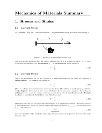
Mechanics of Materials Summary1. Stresses and Strains1.1Normal StressLet’s consider a fixed rod. This rod has length L. Its cross-sectional shape is constant and has area A.Figure 1.1: A rod with a normal force applied to it.Now we will start pulling the rod. We apply a tensional load N to it, as shown in figure 1.1. At everypoint in the rod will then be a normal force N . The normal stress is now defined asσ 1.2N.A(1.1.1)Normal StrainDue to the normal force, the rod will elongate in its longitudinal direction. Its length will change by adisplacement δ. The strain is now defined asε δ.L(1.2.1)There is a relation between the normal stress and the strain. This relation is usually given by a stressstrain diagram. However, it is hard to do calculations if you only have a diagram. But as long asyielding does not occur, the relation between σ and ε is linear. The E-modulus (also called Young’smodulus or modulus of elasticity) is then defined such thatE σ.ε(1.2.2)The normal force will not only cause the rod to elongate in its longitudinal direction. It will also contractin its axial direction. There is a relation between the longitudinal strain εlongitudinal and its axial strainεaxial . This relation isεaxialν .(1.2.3)εlongitudinalHere ν is Poisson’s ratio. Due to the minus sign, Poisson’s ratio is always positive. Its value will usuallybe around 0.3.1
1.3Rod ElongationLet’s suppose we know the dimensions (A and L), properties (E) and loading conditions (N ) of a rod.Can we find the elongation δ? In fact, we can. Using the definitions we just made, we find thatδ NL.EA(1.3.1)There is a fundamental assumption behind this equation. We have assumed that the normal force N ,the E-modulus E and the cross-sectional area A are constant throughout the length of the rod. If this isnot the case, things will be a bit more difficult. Now we can find the displacement usingZ LNdx.(1.3.2)δ 0 EANote that for constant N , E and A this equation reduces back to equation (1.3.1).1.4Shear StressNow let’s not pull the rod. Instead, we put a load on it as shown in figure 1.2. This will cause a shearforce to be present in the rod.Figure 1.2: A rod with a shear force applied to it.Just like a normal force results in a normal stress, so will a shear force result in a shear stress. The shearstress τ isVτ .(1.4.1)AThis equation isn’t entirely exact. This is because the shear stress isn’t constant over the entire crosssection. We will examine shear stress in a later chapter.1.5Shear StrainA shear force also causes some kind of deformation. This time we will have shear strain. Shear straincan be defined as the change of an angle that was previously 90 . So shear strain is an angle (with unitradians). Since the idea of the shear strain can be a little bit hard to grasp, figure 1.3 is present to clarifyit a bit.There is a relation between the shear stress τ and the shear force γ. This relation is given byG 2τ,γ(1.5.1)
Figure 1.3: Clarification of the shear strain.where G is the shear modulus (also called shear modulus of elasticity or modulus of rigidity).Just like the E-modulus, the shear modulus is a material property. There also is a relation between theE-modulus and the shear modulus. This relation involves Poisson’s ratio ν. In fact, it isE 2 (1 ν) .G3(1.5.2)
2. Thermal Effects and Prestress2.1Heating an ObjectWhen an object is heated, it expands. An important parameter during this expansion if the coefficientof thermal expansion α. The strain due to thermal effects, the so-called thermal strain εT , can thenbe found usingεT α Tand alsoδT Lα T,(2.1.1)where T is the temperature difference and δT is the elongation of the bar due to this temperaturedifference.The value of T is not always equal for different points on the rod. If the heating is performed unevenly,it is more difficult to find δT . This time we have to useZ LZ LδT εT dx α T dx.(2.1.2)02.20Heating a Blocked RodNow suppose we have a rod, clamped on both sides. Let’s heat this rod. It tries to expand, but the wallswon’t make way for this expansion. Instead, the walls exert a compressive force N on the rod to keep itat its original length. The entire situation is shown in figure 2.1.Figure 2.1: The heating of a blocked rod.The bar retains its original length. So the total strain is 0. This strain consists of a thermal part and apart due to the normal force. So we find thatεT εN 0 α T N 0.EA(2.2.1)Note that the minus sign is present because the force N is compressive. The force N in the originalequation (from the previous chapter) was tensional. The above equation is called a compatibilityequation. It is the extra equation necessary to solve the problem.Now the force exerted by the walls can be found. Also the stress due to this thermal effect can be found.They areN(2.2.2)N EAα TandσT Eα T EεT .AOnce more the minus sign is present, for the same reason as in the last equation.4
2.3PrestressIn the previous chapter we saw that there was a constant force acting on the rod. It was as if the rodwas too small to fit between the walls. This gives us an idea.Let’s take a rod that is only slightly too long to fit between two walls. When we want to install the rod,we first need to compress it (to shorten it). Let’s suppose a (compressive) prestress force Q is necessaryfor this. After the rod has been placed, there will always be a certain stress in the rod. This prestressσP is then equal toQ(2.3.1)σP .AThe elongation of the bar due to this prestress then isZδP 0LσPdx EZ0LQdx.AE(2.3.2)There are minus signs again because Q is a compressive force. Note that this is logical, as we havecompressed the bar, so δP must be negative as well.2.4The TurnbuckleNow we don’t want to place a rod between two walls, but a cable. Installed in this cable is a turnbuckle.This is a device with which you can shorten the cable slightly. It does this by (sort of) removing a pieceof the cable.If you turn a turnbuckle once, it removes a length p from one side of the cable, where p is the turnbucklepitch. However, a turnbuckle has a cable on both of its sides (both left and right). So one turn willcause a shortening of the rope of 2p. In general, we can now say that the displacement of the rope dueto the turnbuckle isδP 2np,(2.4.1)where n is the amount of turns you have made. The minus sign is present because the turnbuckle decreasesthe length of the rope.Figure 2.2: Situation sketch of the cable with the turnbuckle.Let’s now install a cable between two walls, as shown in figure 2.2. Initially this cable is simply hanginghorizontally, without any stress in it. Then we start turning the turnbuckle. Since the cable is fixed tothe walls, it needs to retain its original length. This causes the walls to exert a force on the cables. Thisforce can be found usingNL 0,(2.4.2)δP δN 0 2np EAwhere N is the tensional force exerted by the walls on the cable. It follows thatN 2npEALandσP 5N2np E.AL(2.4.3)
3. Mechanics of Materials Theory3.1Thin-Walled StructuresBefore we venture further into the depths of mechanics of materials, we first need to discuss some basicideas. The first idea we will discuss is that of thin-walled structures. Let’s consider the I-beam crosssection shown in figure 3.1. Such a cross-section is often used in constructions for reasons we will discoverin later chapters.Figure 3.1: Another example of a cross-sectional shape: an I-beam.We can try to calculate the area of this I-beam. We see a horizontal part of the beam with width w, avertical part with height h and another horizontal part with height w. So we might initially think thatA wt ht wt 2wt ht.(3.1.1)However, now we’ve counted the overlapping parts twice. If we keep those into account, we will getA wt (h 2t)t wt 2wt ht 2t2 .(3.1.2)The second way of calculating things is more exact. However, as cross-sectional shapes get more complicated, this second way will become rather difficult.Now let’s look at the differences. The difference between the two methods is in this case 2t2 . Usually thethickness t is small compared to the width w and height h. The quantity t2 is then very small. If this isthe case, we say we have a thin-walled structure. We then may neglect any factors with t2 and such.So the key idea is as follows: In thin-walled structures you do not have to consider the very small parts(with high powers of t). There will be no terms like (h 2t) and such. These terms all simplify to justh. By using this assumption, the analysis of many cross-sections is simplified drastically.3.2Center of Gravity - Method 1In the next chapters we will be analyzing forces in beams. The way in which the beams behave, stronglydepends on the shape of its cross-section. So the coming couple of paragraphs we will examine thecross-sections of beams.A first thing which we need to find is the position of the center of gravity of a cross-section. Thisposition has coordinates (x, y). The values of x and y can be found usingZZ11x x dAandy y dA.(3.2.1)A AA ATo explain how to use these equations, we use an example. Let’s consider the rectangle shown in figure3.2.6
Figure 3.2: An example of a cross-sectional shape: a square.The value of x can be found usingZZ w1 1 2111h x dx x x dA hw w.A Ahw 0hw 22(3.2.2)Identically we can find that y 12 h. So the center of gravity is exactly in the middle of the rectangle, aswas expected.3.3Center of Gravity - Method 2The method of the previous paragraph has a few downsides. For complicated cross-sections it is oftenvery hard to evaluate the integral. Cross-sectional shapes often consist of an amount of sub-shapes, ofwhich you already know the position of the center of gravity. It would be much easier to use that fact tofind the position of the center of gravity.Now we will do exactly that. Let’s define Atot as the total area of the cross-section. We can now find xand y using1 X1 Xx y xi Aiandyi Ai ,(3.3.1)AtotAtotwhere xi , yi is the position of the center of gravity of every subpart i and Ai the corresponding area. Forthe shape of figure 3.1 (the I-beam) we will thus gety 1 2h t wht1 X111yi Ai h (ht) (h)(wt) 2 h.(0)(wt) Atot2wt ht22wt ht2(3.3.2)The center of gravity is exactly in the middle. We could have expected that, since the structure issymmetric. Instead of having to integrate things, we only need to add up things with this method.That’s why this method is mostly used to find the center of gravity of a cross-section.3.3.1Moment of Inertia - Method 1A quantity that often occurs when analyzing bending moments isZZIx (y yr )2 dAandIy (x xr )2 dA.A(3.3.3)AHere the point xr , yr is a certain reference point. The parameters Ix and Iy are called the secondmoment of inertia about the x-axis/y-axis. The second moment of inertia is also called the areamoment of inertia, or shortened it is just moment of inertia. The moment of inertia is alwaysminimal if you calculate it with respect to the center of gravity (so if xr x and yr y).7
To see how these equations work, we will find the value Ix for a rectangle, as shown in figure 3.2. We dothis with respect to the center of gravity. We thus get" 2 3 # hZ h Z11112y h w dx Ix (y y) dA w y hwh3 .(3.3.4) 232120A0Identically, we find that the moment of inertia about the y-axis is Iy 1312 hw .Next to Ix and Iy , there is also the polar moment of inertia Ip , defined asZ Ip x2 y 2 dA Ix Iy .(3.3.5)AThis quantity is also often denoted as J.3.4Moment of Inertia - Method 2Evaluating an integral every time we need to know a moment of inertia is rather annoying. There mustbe a more simple method. It would be great if we can evaluate a cross-section part by part. Well, whycan’t we do this?There is a good reason for that. A moment of inertia is always with respect to a certain reference point.We can’t add up the moment of inertias of parts with different reference points. So what we need to do,is make the reference points for every part equal. We need to move them! More specifically, we need tomove them to the center of gravity of the entire cross-section. How do we do this?There is a rule, called Steiner’s rule (also called the parallel axis theorem), with which you can movethe reference point. Suppose we have the moment of inertia with respect to the center of gravity andwant to know it with respect to another point xr , yr . The equations we can then use are2Ixr Ixcog A (yr ycog )and2Iyr Iycog A (xr xcog ) .(3.4.1)So if we move the reference point away from the center of gravity by a distance d in a certain direction,then the moment of inertia for the corresponding axis increases by Ad2 . This term Ad2 is called Steiner’sterm.So, taking into account the Steiner’s term, we can derive another expression for the moment of inertia.It will become X X 22Ixtot Ixi Ai (ycogtot ycogi )andIytot Iyi Ai (xcogtot xcogi ) . (3.4.2)If we apply this to the I-shaped beam of figure 3.1, we find 2 !11111 3wt (wt)h th3 wth2 th3 .Ix 212212212(3.4.3)We don’t have a Steiner’s term for the vertical part of the beam (the so-called web). This is becausethe center of gravity of this part coincides with the center of gravity of the whole cross-section. Alsonote that we have ignored the term involving t3 at the horizontal parts (the flanges). This is becausewe assumed we are dealing with a thin-walled structure.3.5The Moment of Inertia for Common Cross-Sectional ShapesTo apply the method of the previous paragraph, we need to know the moment of inertia for a couple ofshapes. Some of them are given here. The following moment of inertias are with respect to the center ofgravity of that cross-section. For that reason, the position of the center of gravity is also given.8
A rectangle, with width w and height h. The center of gravity is in its center (at height 21 h andwidth 12 w). The moment of inertias areIx 1wh312andIy 1hw3 .12(3.5.1) An isosceles triangle, with its base down and tip up. (The tip then lies centered above the base.)The base has width w, and the triangle has height h. The center of gravity now lies on height 31 hand on width 21 w. The moment of inertias areIx 1wh336andIy 1hw3 .48(3.5.2) A circle, with radius R. Its center of gravity lies at the center of the circle. The moment of inertiasare1Ix Iy πR4(3.5.3)4 A tube, with inner radius R1 and outer radius R2 . Its center of gravity lies at the center of thetube. The moment of inertias areIx Iy 9 1π R24 R144(3.5.4)
4. Normal Forces and Bending Moments4.1Introduction to BendingLet’s consider a beam. We can bend this beam with only a bending moment M . This form of bending(bending without any normal forces) is called pure bending. But what will happen to the beam underpure bending? To find that out, we have to look at a small part dx of the beam, as is done in figure 4.1.Figure 4.1: Deformation of a small part of beam under bending.We see that one part of the beam (in this case the top part) elongates, while the other part is beingcontracted. So part of the beam has tensile stress, while the other has compressive stress. Also, there issome part in the beam without any stresses. This part is called the neutral axis (also called neutralline).Let’s see if we can find an expression for the stress. For that, we first ought to consider the strain. Thisstrain depends on the bend radius R and the position in the beam y. Here y is the distance from theneutral axis. We will find that the strain due to a bending moment isεM (y) Lnew Lold LoldR yR dxdx dx y.R(4.1.1)For some reason engineers don’t like to work with a bend radius. Instead, the curvature is defined asκ 1/R. Let’s now assume that no yielding (no permanent deformation) occurs. Then we have as stressEy Eyκ.(4.1.2)RSo the stress varies linearly with the distance y. That’s nice to know! It’s often relatively easy to workwith linear relations. However, our job of analyzing bending is not finished yet.σM εM E 4.2Stress as a Function of the Bending MomentOne thing we would still like to know, is where the neutral axis will be. To find it, we have two pieces ofdata: The equations of the previous paragraph and the fact that there is no normal force (since we aredealing with pure bending). So let’s see if we can find the normal force. This force isZZZZ0 N dF σM dA Eyκ dA Eκy dA.(4.2.1)AAAAE and κ are constant for this cross-section. They are also nonzero, so the integral must be zero. It canbe shown that this is only the case if y is the distance from the center of gravity of the cross-section. Sothe neutral line is the center of gravity of the cross-section!10
That’s very nice to know, but we still can’t calculate much. Although we know the stress as a functionof the curvature κ, this curvature is usually unknown. Can we express the stress as a function of thebending moment M ? In fact, we can. This bending moment can be found usingZZM y dF Eκy 2 dA EκI,(4.2.2)AAwhere I is the moment of inertia about the horizontal axis of the cross-section. The minus sign in theequation is present due to the sign convention of the bending moment. A couple of engineers decidedthat to bend the beam as shown in figure 4.1, a negative bending moment was required.So now we have expressed the curvature κ as a function of the bending moment. Combining this withthe equations of the previous paragraph, we find the equation for the stress under pure bending (theso-called flexure formula). It isMy.(4.2.3)σM IWe can derive another important fact from this equation. We can find where maximum stress occurs.M and I are constant for a cross-section. So maximum stress occurs if y is maximal. This is thus at thetop/bottom of the cross-section.4.3Adding a Normal ForceSo now we know the normal stress in a beam when it is subject to only a bending moment. What happenswhen we subject a beam to a normal force N ? Well, if there is only a normal force, then the normalstress is easy to find. It isN(4.3.1)σN .ABut what do we do if we have a normal force and a bending moment simultaneously? The answer to thatquestion is quite simple. We add the stress up. So the total stress σT then becomesσT σN σM NMy .AI(4.3.2)The principle used in this relation is the principle of superposition.Figure 4.2: Stress diagram for different loading cases.Now let’s examine the stress in a beam. We do this using the stress diagrams of figure 4.2. When therewas only a bending moment, the neutral axis was at the center of gravity of the cross-section. Applyinga normal force shifts the neutral line by a distance d. This distance can be found usingNMd 0AI d NI.MA(4.3.3)When the normal force gets sufficiently big, the neutral line may move outside of the cross-section. Thenthere isn’t any part in the beam anymore without stress.11
5. Shear Stress and Shear Flow5.1The Shear Stress EquationNow we have expressions for the normal stress caused by bending moments and normal forces. It wouldbe nice if we can also find an expression for the shear stress due to a shear force. So let’s do that.Figure 5.1: An example cross-section, where a cut has been made.We want to know the shear stress at a certain point. For that, we need to look at the cross-section of thebeam. One such cross-section is shown in figure 5.1. To find the shear stress at a given point, we make acut. We call the thickness of the cut t. We take the area on one side of the cut (it doesn’t matter whichside) and call this area A0 . Now it can be shown thatZVτ y dA.(5.1.1)It A0Here y is the vertical distance from the center of gravity of the entire cross-section. (Not just the partA0 !) Let’s evaluate this integral for the cross-section. We find that! ZZ h/2Z h/2 tV1VV 1 2y dA h t wht .(5.1.2)τ yt dy yw dy It A0ItIt 820h/2Note that we have used the thin-walled structure principle in the last step.So now we have found the shear stress. Note that this is the shear stress at the position of the cut! Atdifferent places in the cross-section, different shear stresses are present.One thing we might ask ourselves now is: Where does maximum shear stress occur? Well, it can beshown that this always occurs in the center of gravity of the cross-section. So if you want to calculatethe maximum shear stress, make a cut through the center of gravity of the cross-section. (An exceptionmay occur if torsion is involved, but we will discuss that in a later chapter.)5.2A Slight SimplificationEvaluating the integral of (5.1.1) can be a bit difficult in some cases. To simplify things, let’s define Q asZQ y dA,(5.2.1)A0implying thatτ VQ.It12(5.2.2)
We have seen this quantity Q before. It was when we were calculating the position of the center of gravity.And we had a nice trick back then to simplify calculations. We split A0 up in parts. Now we haveXQ yi A0i ,(5.2.3)with A0i the area of a certain part and yi the position of its center of gravity. We can apply this to thecross-section of figure 5.1. We would then get 111Vτ hht h (wt) .(5.2.4)It422Note that this is exactly the same as what we previously found (as it should be).5.3Shear FlowLet’s define the shear flow q asVQ.(5.3.1)INow why would we do this? To figure that out, we take a look at the shear stress distribution and theshear flow distribution. They are both plotted in figure 5.2.q τt Figure 5.2: Distribution of the shear stress and the shear flow over the structure.We see that the shear stress suddenly increases if the thickness decreases. This doesn’t occur for the shearflow. The shear flow is independent of the thickness. You could say that, no matter what the thicknessis, the shear flow flowing through a certain part of the cross-section stays the same.5.4BoltsSuppose we have two beams, connected by a number of n bolts. In the example picture 5.3, we haven 2. These bolts are placed at intervals of s meters in the longitudinal direction, with s being thespacing of the bolts.Figure 5.3: Example of a cross-section with bolts.13
Suppose we can measure the shear force Vb in every bolt. Let’s assume that these shear forces are equalfor all bolts. (In asymmetrical situations things will be a bit more complicated, but we won’t go intodetail on that.) The shear flow in all the bolts together will then beqb nVb.s(5.4.1)Now we can reverse the situation. We can calculate the shear flow in all bolts together using the methodsfrom the previous paragraph. In our example figure 5.3, we would have to make a vertical cut throughboth bolts. Now, with the above equation, the shear force per bolt can be calculated.5.5The Value of Q for Common Cross-Sectional ShapesIt would be nice to know the maximum values of Q for some common cross-sectional shapes. This couldsave us some calculations. If you want to know Qmax for a rather common cross-section, just look it upin the list below. A rectangle, with width w and height h.Qmax wh28andτmax 3V3 V .2A2 wh(5.5.1)Qmax 2 3R3andτmax 4V4 V .3A3 πR2(5.5.2) A circle with radius R. A tube with inner radius R1 and outer radius R2 .Qmax 2R23 R133andτmax V4R22 R1 R2 R12.223 π (R2 R1 )R22 R12(5.5.3) A thin-walled tube with radius R and thickness t.Qmax 2R2 tand14τmax 2VV .AπRt(5.5.4)
6. Torsion6.1Introduction to TorsionWe have now dealt with normal forces, shear forces and bending moments. Only torsion is left.Torsion is caused by a torque T . This torque causes the bar to twist by an angle φ; the so-called angleof twist. A visualization of this is given in figure 6.1.Figure 6.1: A bar with a torque T applied to it.Another important angle is the rotation per meter θ, defined asθ φ.L(6.1.1)Here L is the length of the bar.In this chapter, we will mainly consider pure torsion. This is when the torque acts on the center ofgravity of the cross-section. At the end we will combine this with a shear force.6.2The Torsion FormulaLet’s consider a beam with a circular cross-section. What happens when we put a torque T on it? Thetorque causes a shear stress τ in the bar. And where there is shear stress, there is shear strain. Thisshear strain γ is given byγ ρθ.(6.2.1)The variable ρ is the distance with respect to the center of gravity of the bar. The shear stress can nowbe found usingτ Gγ Gρθ.(6.2.2)However, usually θ isn’t known. But we usually do know the torque T that acts on a bar. The torquecan also be found usingZZT ρτ dA Gθρ2 dA GθIp .(6.2.3)AACombining the above equations, we find an expression for the shear stress. Namely,τ Tρ.Ip(6.2.4)This equation is known as the torsion formula. Let’s take a close look at this equation. It turns outthat the shear stress τ increases as we go further from the center of gravity of the cross-section. Somaximum shear stress occurs at the edges of the cross-section.15
One final thing we would like to know is the angle of twist. We can find it usingZ06.3LZθ dx φ 0Lτdx GρZL0TTLdx .GIpGIp(6.2.5)Closed Thin-Walled Cross-SectionsPreviously we considered a circular cross-section. Now we will look at closed thin-walled crosssections. A cross-section is closed if it consists of an uninterrupted curve. Let’s define Lm as the lengthof this curve. Also, Am is the mean enclosed area (the area which the curve encloses). It can now beshown that the shear flow is given byT.(6.3.1)q 2AmThe shear stress at a given point in the cross-section can now be found usingT,2tAmτ (6.3.2)where t is the thickness at that point of the cross-section.To find the angle of twist, we can still use the familiar equationφ TL.GIp(6.3.3)There is, however, one slight problem. It is usually rather difficult to find the polar moment of inertia forthese cross-sections in the conventional way. Luckily, there is another equation which we can use. It is4A2Ip H Lm m .1t ds0(6.3.4)HThe sign means that the integration must be performed along the entire boundary. If the thickness tvaries only in steps (which it usually does), then you can also useIp P4A2m.(Lmi /ti )(6.3.5)Here ti is the thickness at a certain part of the cross-section and Lmi is the length of that part.6.4Combining Shear Forces and TorsionWhat do we do if we have both a shear force and a torque acting on a beam? In that case, we can usethe principle of superposition. First find the shear stress distribution for the beam when only the shearforce is present. Then find the shear stress distribution for the beam when only the torque is present.(Keep in mind the direction of the shear stress!) Then simply add it all up to find the real shear stressdistribution. Sounds easy, doesn’t it?16
7. Bending Deflection7.1The Differential EquationsIn the last chapter we saw the effect of a torque: A twist angle. What is the effect of bending a beam?There are two things that are of interest: The beam rotation θ and the deflection u δ.To be able to analyze this problem without having awfully difficult equations, we have to assume thatthe beam rotations and deflections are small. If we make that assumption, we can derive five equations.These ared4 udx4d3 uEIu000 EI 3dxd2 u00EIu EI 2 EIκdxdu0u dxu EIu0000 EI(7.1.1)V (x) (7.1.2)M (x) θ(x) δ(x) q(x)(7.1.3)(7.1.4)(7.1.5)Let’s discuss the sign convention. The distributed load q is assumed to act downward, and so is thevertical force V . The moment M is assumed to be clockwise. The rotation θ is assumed to be clockwiseas well. Finally, the displacement is positive when the beam is deflected downward.So, if we have a distributed load q acting on a beam, all we have to do is integrate four times and wehave the deflection. It sounds easy, but actually, it isn’t easy at all. Not only is it annoying to integratefour times. But during every integration, a new constant pops up. That’ll be a lot of constants! Youneed to solve for these constants using boundary conditions.So, it’s a lot of work. And it’s very easy to make an error. I can imagine you’ve got better things to do.So let’s look for an easier method to find the rotation/deflection of a beam.7.2Vergeet-Me-Nietjes/Forget-Me-NotsThe second (and mostly used) method to determine deflections is by considering standard load types.Sounds vague so far? Well, the idea is as follows. We have a clamped beam. On this beam is a certainload type working. The load types we will be considering are shown in figure 7.1.Figure 7.1: The three load types we will be considering.These are the three standard load types. The rotation and displacement of the tip has been calculated forthese examples. The results are shown in table 7.1. These equations are called the vergeet-me-nietjes17
(in Dutch) or the forget-me-nots (in English), named after the myosotis flower. They are thereforesometimes also called the myosotis equations.Load type:A distributed load q, pointing downwardA single force P , pointing downwardA single moment M , applied CCWθ:δ:qL36EIP L22EIMLEIqL48EIP L33EIM L22EITable 7.1: The vergeet-me-nietjes/forget-me-nots.7.3Applying the Forget-Me-NotsSo, how do we apply the forget-me-nots? Just follow the following steps: Split the beam up in segments. Every segment should be one of the standard load types. For every segment, do the following:– Let’s call the left side of the segment point A and the right side point B. First find the forcesand moments acting on B. (Don’t forget the internal forces in the beam!)– Now express the rotation and displacement in B as a function of the rotation and displacementin A. For that, use the equationsθBδBqAB L3ABPB L2ABMB LAB ,6EI2EIEIqAB L4ABPB L3ABMB L2AB δA LAB θA .8EI3EI2EI θA (7.3.1)(7.3.2)(7.3.3)An important part is the term LθA at the end of the last equation. This term is present dueto the so-called wagging tail effect. It is often forgotten, so pay special attention to it.To demonstrate this method, we consider an example. Let’s take a look at figure 7.2. Can we determinethe displacement at point C?Figure 7.2: An example problem for the forget-me-nots.It’s quite clear that we need to split
Mechanics of Materials Summary 1. Stresses and Strains 1.1 Normal Stress Let's consider a fixed rod. This rod has length L. Its cross-sectional shape is constant and has area A. Figure 1.1: A rod with a normal force applied to it. Now we will start pulling the rod. We apply a tensional load N to it, as shown in figure 1.1. At every