Transcription
Flight Dynamics Summary1. IntroductionIn this summary we examine the flight dynamics of aircraft. But before we do that, we must examinesome basic ideas necessary to explore the secrets of flight dynamics.1.11.1.1Basic conceptsControlling an airplaneTo control an aircraft, control surfaces are generally used. Examples are elevators, flaps and spoilers.When dealing with control surfaces, we can make a distinction between primary and secondary flightcontrol surfaces. When primary control surfaces fail, the whole aircraft becomes uncontrollable.(Examples are elevators, ailerons and rudders.) However, when secondary control surfaces fail, theaircraft is just a bit harder to control. (Examples are flaps and trim tabs.)The whole system that is necessary to control the aircraft is called the control system. When a controlsystem provides direct feedback to the pilot, it is called a reversible system. (For example, when usinga mechanical control system, the pilot feels forces on his stick.) If there is no direct feedback, then wehave an irreversible system. (An example is a fly-by-wire system.)1.1.2Making assumptionsIn this summary, we want to describe the flight dynamics with equations. This is, however, very difficult.To simplify it a bit, we have to make some simplifying assumptions. We assume that . . . There is a flat Earth. (The Earth’s curvature is zero.) There is a non-rotating Earth. (No Coriolis accelerations and such are present.) The aircraft has constant mass. The aircraft is a rigid body. The aircraft is symmetric. There are no rotating masses, like turbines. (Gyroscopic effects can be ignored.) There is constant wind. (So we ignore turbulence and gusts.)1.21.2.1Reference framesReference frame typesTo describe the position and behavior of an aircraft, we need a reference frame (RF). There are severalreference frames. Which one is most convenient to use depends on the circumstances. We will examinea few.1
First let’s examine the inertial reference frame FI . It is a right-handed orthogonal system. Itsorigin A is the center of the Earth. The ZI axis points North. The XI axis points towards thevernal equinox. The YI axis is perpendicular to both the axes. Its direction can be determinedusing the right-hand rule. In the (normal) Earth-fixed reference frame FE , the origin O is at an arbitrary location onthe ground. The ZE axis points towards the ground. (It is perpendicular to it.) The XE axis isdirected North. The YE axis can again be determined using the right-hand rule. The body-fixed reference frame Fb is often used when dealing with aircraft. The origin of thereference frame is the center of gravity (CG) of the aircraft. The Xb axis lies in the symmetryplane of the aircraft and points forward. The Zb axis also lies in the symmetry plane, but pointsdownwards. (It is perpendicular to the Xb axis.) The Yb axis can again be determined using theright-hand rule. The stability reference frame FS is similar to the body-fixed reference frame Fb . It is rotatedby an angle αa about the Yb axis. To find this αa , we must examine the relative wind vectorVa . We can project this vector onto the plane of symmetry of the aircraft. This projection is thenthe direction of the XS axis. (The ZS axis still lies in the plane of symmetry. Also, the YS axis isstill equal to the Yb axis.) So, the relative wind vector lies in the XS YS plane. This reference frameis particularly useful when analyzing flight dynamics. The aerodynamic (air-path) reference frame Fa is similar to the stability reference frame FS .It is rotated by an angle βa about the ZS axis. This is done, such that the Xa axis points in thedirection of the relative wind vector Va . (So the Xa axis generally does not lie in the symmetryplane anymore.) The Za axis is still equation to the ZS axis. The Ya axis can now be found usingthe right-hand rule. Finally, there is the vehicle reference frame Fr . Contrary to the other systems, this is a lefthanded system. Its origin is a fixed point on the aircraft. The Xr axis points to the rear of theaircraft. The Yr axis points to the left. Finally, the Zr axis can be found using the left-hand rule.(It points upward.) This system is often used by the aircraft manufacturer, to denote the positionof parts within the aircraft.1.2.2Changing between reference framesWe’ve got a lot of reference frames. It would be convenient if we could switch from one coordinate systemto another. To do this, we need to rotate reference frame 1, until we wind up with reference frame 2. (Wedon’t consider the translation of reference frames here.) When rotating reference frames, Euler anglesφ come in handy. The Euler angles φx , φy and φz denote rotations about the X axis, Y axis and Z axis,respectively.We can go from one reference frame to any other reference frame, using at most three Euler angles. Anexample transformation is φx φy φz . In this transformation, we first rotate about the X axis,followed by a transformation about the Y axis and the Z axis, respectively. The order of these rotationsis very important. Changing the order will give an entirely different final result.1.2.3Transformation matricesAn Euler angle can be represented by a transformation matrix T. To see how this works, we considera vector x1 in reference frame 1. The matrix T21 now calculates the coordinates of the same vector x2in reference frame 2, according to x2 T21 x1 .2
Let’s suppose we’re only rotating about the X axis. In this case, the transformation matrix T21 is quitesimple. In fact, it is 100 (1.2.1)T21 0 cos φxsin φx .0 sin φx cos φxSimilarly, we can rotate aboutrespectively, cos φy T21 0sin φythe Y axis and the Z axis. In this case, the transformation matrices are, 0 sin φy 10 0 cos φy andT21cos φz sin φz0sin φzcos φz0 0 0 .1(1.2.2)A sequence of rotations (like φx φy φz ) is now denoted by a sequence of matrix multiplicationsT41 T43 T32 T21 . In this way, a single transformation matrix for the whole sequence can be obtained.Transformation matrices have interesting properties. They only rotate points. They don’t deform them.For this reason, the matrix columns are orthogonal. And, because the space is not stretched out either,these columns must also have length 1. A transformation matrix is thus orthogonal. This implies thatTT 121 T21 T12 .1.2.4(1.2.3)Transformation examplesNow let’s consider some actual transformations. Let’s start at the body-fixed reference frame Fb . If werotate this frame by an angle αa about the Y axis, we find the stability reference frame FS . If we thenrotate it by an angle βa about the Z axis, we get the aerodynamic reference frame Fa . So we can findthat cos αa 0 sin αacos βasin βa 0cos βasin βa 0 (1.2.4)xa sin βa cos βa 0 xS sin βa cos βa 0 010 xb .001 sin αa 0 cos αa001By working things out, we can thus find that cos βa cos αa Tab sin βa cos αa sin αasin βacos βa0 cos βa sin αa sin βa sin αa .cos αa(1.2.5)We can make a similar transformation between the Earth-fixed reference frame FE and the body-fixedreference frame Fb . To do this, we first have to rotate over the yaw angle ψ about the Z axis. We thenrotate over the pitch angle θ about the Y axis. Finally, we rotate over the roll angle ϕ about the Xaxis. If we work things out, we can find that cos θ cos ψcos θ sin ψ sin θ TbE sin ϕ sin θ cos ψ cos ϕ sin ψ sin ϕ sin θ sin ψ cos ϕ cos ψ sin ϕ cos θ .(1.2.6)cos ϕ sin θ cos ψ sin ϕ sin ψ cos ϕ sin θ sin ψ sin ϕ cos ψ cos ϕ cos θNow that’s one hell of a matrix . . .3
1.2.5Moving reference framesLet’s examine some point P . This point is described by vector rE in reference frame FE and by rb inreference frame Fb . Also, the origin of Fb (with respect to FE ) is described by the vector rEb . So wehave rE rEb rb .Now let’s examine the time derivative of rE in FE . We denote this bydrEdt EdrEbdt Edrbdt.drEdt. It is given byE(1.2.7)ELet’s examine the terms in this equation. The middle term of the above equation simply indicates themovement of Fb , with respect to FE . The right term is, however, a bit more complicated. It indicatesthe change of rb with respect to FE . But we usually don’t know this. We only know the change of rbin Fb . So we need to transform this term from FE to Fb . Using a slightly difficult derivation, it can beshown thatdrbdrb ΩbE rb .(1.2.8)dt Edt bThe vector ΩbE denotes the rotation vector of Fb with respect to FE . Inserting this relation into theearlier equation gives usdrEdrEbdrb ΩbE rb .(1.2.9)dt Edt Edt bThis is quite an important relation, so remember it well. By the way, it holds for every vector. So insteadof the position vector r, we could also take the velocity vector V.Finally, we note some interesting properties of the rotation vector. Given reference frames 1, 2 and 3, wehaveΩ12 Ω21andΩ31 Ω32 Ω21 .(1.2.10)4
2. Deriving the equations of motionThe flight dynamics of an aircraft are described by its equations of motion (EOM). We are going toderive those equations in this chapter.2.12.1.1ForcesThe basic force equationTo derive the equations of motion of an aircraft, we start by examining forces. Our starting point inthis is Newton’s second law. However, Newton’s second law only holds in an inertial reference system.Luckily, the assumptions we have made earlier imply that the Earth-fixed reference frame FE is inertial.(However, Fb is not an inertial reference frame.) So we will derive the equations of motion with respectto FE .Let’s examine an aircraft. Newton’s second law states that Z ZdVp dm ,F dF dt(2.1.1)where we integrate over the entire body. It can be shown that the right part of this equation equalsddt (VG m), where VG is the velocity of the center of gravity of the aircraft. If the aircraft has a constantmass, we can rewrite the above equation intoF mdVG mAG .dt(2.1.2)This relation looks very familiar. But it does imply something very important. The acceleration of theCG of the aircraft does not depend on how the forces are distributed along the aircraft. It only dependson the magnitude and direction of the forces.2.1.2Converting the force equationThere is one slight problem. The above equation holds for the FE reference frame. But we usually workin the Fb reference frame. So we need to convert it. To do this, we can use the relationAG dVGdt EdVGdt ΩbE VG .(2.1.3)bInserting this into the above equation will give F mdVGdt m ΩbE VGbBy the way, in the above equation, we have used that u VG v andw u̇ qw rv m v̇ ru pw .ẇ pv qu(2.1.4) p q .r(2.1.5)ΩbEHere, u, v and w denote the velocity components in X, Y and Z direction, respectively. Similarly, p, qand r denote rotation components about the X, Y and Z axis, respectively.5
2.1.3External forcesLet’s take a look at the forces F our aircraft is subject to. There are two important kinds of forces:gravity and aerodynamic forces. The gravitational force Fgravity is, in fact, quite simple. It is given byhFEgravity 00 mgiT,(2.1.6)where g is the gravitational acceleration. The superscript E indicates that the force is given inthe FE reference frame. However, we want the force in the Fb reference frame. Luckily, we know thetransformation matrix TbE . We can thus find that sin θ E(2.1.7)Fbgravity TbE Fgravity mg sin ϕ cos θ .cos ϕ cos θThe aerodynamic forces Faero are, however, a lot more difficult. For now, we won’t examine them indepth. Instead, we simply say thathiTbbbFb .(2.1.8)XYZaeroBy combining this knowledge with the equation of motion for forces, we find that u̇ qw rv sin θXb b m v̇ ru pw mg sin ϕ cos θ Y .ẇ pv qucos ϕ cos θZb2.22.2.1(2.1.9)MomentsAngular momentumBefore we’re going to look at moments, we will first examine angular momentum. The angular momentum of an aircraft BG (with respect to the CG) is defined asZBG dBG r VP dm,(2.2.1)where we integrate over every point P in the aircraft. We can substituteV P VG drdt ΩbE r.(2.2.2)bIf we insert this, and do a lot of working out, we can eventually find thatBG IG ΩbE .The parameter IG is the inertia tensor, with respect to the CG. It is defined as R RRIx Jxy Jxz(ry2 rz2 )dm (rx ry )dm (rx rz )dmR 2R R IG JxyIy Jyz (rx ry )dm(rx rz2 )dm (ry rz )dm .RRR 2 Jxz JyzIz (rx rz )dm (ry rz )dm(rx ry2 )dm(2.2.3)(2.2.4)We have assumed that the XZ-plane of the aircraft is a plane of symmetry. For this reason, Jxy Jyz 0.This simplifies the inertia tensor a bit.6
2.2.2The moment equationIt is now time to look at moments. We again do this from the inertial reference frame FE . The momentacting on our aircraft, with respect to its CG, is given byZZZd (Vp dm),(2.2.5)MG dMG r dF r dtwhere we integrate over the entire body. Luckily, we can simplify the above relation toMG dBGdt.(2.2.6)EThe above relation only holds for inertial reference frames, such as FE . However, we want to have theabove relation in Fb . So we rewrite it toMG dBGdt ΩbE BG .(2.2.7)bBy using BG IG ΩbE , we can continue to rewrite the above equation. We eventually wind up withMG IGdΩbEdt ΩbE IG ΩbE .(2.2.8)bIn matrix-form, this equation can be written as Ix ṗ (Iz Iy )qr Jxz (pq ṙ) MG Iy q̇ (Ix Iz )pr Jxz (p2 r2 ) .Iz ṙ (Iy Ix )pq Jxz (qr ṗ)(2.2.9)Note that we have used the fact that Jxy Jyz 0.2.2.3External momentsLet’s take a closer look at MG . Again, we can distinguish two types of moments, acting on our aircraft.There are moments caused by gravity, and moments caused by aerodynamic forces. Luckily, the momentscaused by gravity are zero. (The resultant gravitational force acts in the CG.) So we only need to considerthe moments caused by aerodynamic forces. We denote those ashiTMb(2.2.10)N .G,aero L MThis turns the moment equation into Ix ṗ (Iz Iy )qr Jxz (pq ṙ)L 22 Iy q̇ (Ix Iz )pr Jxz (p r ) M .Iz ṙ (Iy Ix )pq Jxz (qr ṗ)N2.32.3.1(2.2.11)Kinematic relationsTranslational kinematicsNow that we have the force and moment equations, we only need to find the kinematic relations for ouraircraft. First, we examine translational kinematics. This concerns the velocity of the CG of the aircraftwith respect to the ground.7
The velocity of the CG, with respect to the ground, is called the kinematic velocity Vk . In the FEreference system, it is described byhVk VNVE VZiT.(2.3.1)In this equation, VN is the velocity component in the Northward direction, VE is the velocity componentin the eastward direction, and VZ is the vertical velocity component. (The minus sign is present because,in the Earth-fixed reference system, VZ is defined to be positive downward.)However, in the Fb reference system, the velocity of the CG, with respect to the ground, is given byhVG uvwiT.(2.3.2)To relate those two vectors to each other, we need a transformation matrix. This gives usVk TEb VG TTbE VG .(2.3.3)This is the translational kinematic relation. We can use it to derive the change of the aircraft position.To do that, we simply have to integrate the velocities. We thus haveZ tZ tZ tx(t) VN dt,y(t) VE dtandh(t) VZ dt.(2.3.4)02.3.200Rotational kinematicsNow let’s examine rotational kinematics. This concerns the rotation of the aircraft. In the FE referencesystem, the rotational velocity is described by the variables ϕ̇, θ̇ and ψ̇. However, in the Fb referencesystem, the rotational velocity is described by p, q and r. The relation between these two triples can beshown to be ϕ̇10 sin θp (2.3.5) q 0 cos ϕ cos θ sin ϕ θ̇ .ψ̇0 sin ϕ cos θ cos ϕrThis is the rotational kinematic relation.q θ̇ and r ψ̇. By the way, we can also 1ϕ̇ θ̇ 0ψ̇0It is interesting to note that, if ϕ θ ψ 0, then p ϕ̇,invert the above relation. We would then get psin ϕ tan θ cos ϕ tan θ (2.3.6)cos ϕ sin ϕ q .sin ϕ/ cos θ cos ϕ/ cos θr8
3. Rewriting the equations of motionThe equations of motion are quite difficult to deal with. To get some useful data out of them, we needto make them a bit simpler. For that, we first linearize them. We then simplify them. And after that,we set them in a non-dimensional form.3.13.1.1LinearizationThe idea behind linearizationLet’s suppose we have some non-linear function f (X). Here, X is the state of the system. It containsseveral state variables. To linearize f (X), we should use a multi-dimensional Taylor expansion. Wethen getf (X) f (X0 ) fX1 (X0 ) X1 fX2 (X0 ) X2 . . . . . . fXn (X0 ) Xn higher order terms. (3.1.1)Here, X0 is the initial point about which we linearize the system. The linearization will only be validclose to this point. Also, the term Xi indicates the deviation of variable Xi from the initial point X0 .When applying linearization, we always neglect higher order terms. This significantly simplifies theequation. (Although it’s still quite big.)3.1.2Linearizing the statesNow let’s apply linearization to the force and moment equations. We start at the right side: the states.We know from the previous chapter thatFxFyFz m(u̇ qw rv), m(v̇ ru pw), m(ẇ pv qu).(3.1.2)(3.1.3)(3.1.4)So we see that Fx f (u̇, q, w, r, v). The state vector now consists of five states. By applying linearization,we find thatFxFyFz m(u 0 q0 w0 r0 v0 ) m( u̇ q0 w w0 q r0 v v0 r), m(v 0 r0 u0 p0 w0 ) m( v̇ r0 u u0 r p0 w w0 p), m(w 0 p0 v0 q0 u0 ) m( ẇ p0 v v0 p q0 u u0 q).(3.1.5)(3.1.6)(3.1.7)We can apply a similar trick for the moments. This would, however, give us quite big expressions. Andsince we don’t want to spoil too much paper (safe the rainforests!), we will not derive those here. Instead,we will only examine the final result in the end.3.1.3Linearizing the forcesNow let’s try to linearize the forces. Again, we know from the previous chapter thatFxFyFz W sin θ X, W sin ψ cos θ Y, W cos ψ cos θ Z,9(3.1.8)(3.1.9)(3.1.10)
where the weight W mg. We see that this time Fx f (θ, X). Also, Fy f (ψ, θ, Y ) and FZ f (ψ, θ, Z). It may seem that linearization is easy this time. However, there are some problems.The problems are the forces X, Y and Z. They are not part of the state of the aircraft. Instead theyalso depend on the state of the aircraft. And they don’t only depend on the current state, but on theentire history of states! (For example, a change in angle of attack could create disturbances at the wing.These disturbances will later result in forces acting on the tail of the aircraft.)How do we put this into equations? Well, we say that X is not only a function of the velocity u, butalso of all its derivatives u̇, ü, . . . And the same goes for v, w, p, q and r. This gives us an infinitelybig equation. (Great. . . .) But luckily, experience has shown that we can neglect most of these timederivatives, as they aren’t very important. There are only four exceptions. v̇ strongly influences thevariables Y and N . Also, ẇ strongly influences Z and M . We therefore say thatFx f (θ, X)Fy f (ψ, θ, Y )Fz f (ψ, θ, Z)withwithwithX f (u, v, w, p, q, r, δa , δe , δr , δt ),Y f (u, v, w, v̇, p, q, r, δa , δe , δr ),Z f (u, v, w, ẇ, p, q, r, δa , δe , δr , δt ).(3.1.11)(3.1.12)(3.1.13)When creating the Taylor expansion, we have to apply the chain rule. We then find thatFx (X) Fx (X0 ) W cos θ0 θ Xu u Xv v Xw w Xp p . . . Xδt δt , (3.1.14)Fy (X) Fy (X0 ) W sin ψ0 sin θ0 θ W cos ψ0 cos θ0 ψ Yv̇ v̇ . . . Yδr δr , (3.1.15)Fz (X) Fz (X0 ) W cos ψ0 sin θ0 θ W sin ψ0 cos θ0 ψ Zẇ ẇ . . . Zδt δt . (3.1.16)Now that’s one big Taylor expansion. And we haven’t even written down all terms of the equation.(Note the dots in the equation.) By the way, the term Xu indicates the derivative X/ u. Similarly,Xv X/ v, and so on.You may wonder what δa , δe , δr and δt are. Those are the settings of the aileron, elevator, rudderand thrust. These settings of course influence the forces acting on the aircraft. We will examine thosecoefficients later in more detail. (You may also wonder, why doesn’t Y depend on the thrust setting δt ?This is because we assume that the direction of the thrust vector lies in the plane of symmetry.)3.23.2.1SimplificationSymmetry and asymmetryLet’s try to simplify that monstrocity of an equation of the previous part. To do that, we have to applyseveral tricks. The most important one, is that of symmetry and asymmetry.We can make a distinction between symmetric and asymmetric forces/deviations. The symmetric deviations (the deviations which don’t break the symmetry) are u, w and q. The symmetric forces/momentsare X, Z and M . Similarly, the asymmetric deviations are v, p and r. The asymmetric forces/momentsare Y , L and N .It can now be shown that there is no coupling between the symmetric and the asymmetric properties.(That is, as long as the deviations are small.) In other words, X is uneffected by v, p and r. ThusXv Xp Xr 0. The same trick works for the other forces and moments as well. This causes a lotof terms to disappear in the force equations.10
3.2.2Simplifying the force equationsThere is also another important trick we use, when simplifying the force equations. We assume that theaircraft is flying in a steady symmetric flight. This means thatu0 6 0 u̇0 0v0 0 v̇0 0w0 6 0 ẇ0 0p0 0 ṗ0 0 ϕ0 0 ϕ̇0 0 X0 6 0q0 0 q̇0 0 θ0 6 0 θ̇0 0 Y0 0r0 0 ṙ0 0 ψ0 6 0 ψ̇0 0 Z0 6 0Ẋ0 0,Ẏ0 0,Ż0 0.(3.2.1)This greatly simplifies the Fx (X0 ), Fy (X0 ) and Fz (X0 ) terms.Now it is finally time to apply all these simplifications and tricks. It will give us the force equations forsmall deviations from a steady symmetric flight. These equations are W cos θ0 θ Xu u Xw w Xq q Xδe δe Xδt δtW cos θ0 ψ Yv v Yv̇ v̇ Yp p Yr r Yδa δa Yδr δr W sin θ0 θ Zu u Zw w Zẇ ẇ Zq q Zδe δe Zδt δt m(u̇ w0 q), m(v̇ u0 r w0 p), m(ẇ u0 q).(3.2.2)(3.2.3)(3.2.4)Of these three equations, the first and the third correspond to symmetric motion. The second equationcorresponds to asymmetric motion.You may wonder, where did all the ’s go to? Well, to simplify our notation, we omitted them. So inthe above equation, all variables indicate the displacement from the initial position X0 .Finally, there is one more small simplification we could do. We haven’t fully defined our reference systemyet. (We haven’t specified where the X axis is in the symmetry plane.) Now let’s choose our referencesystem. The most convenient choice is in this case the stability reference frame FS . By choosing thisframe, we have u0 V and w0 0. (V is the velocity.) This eliminates one more term.3.2.3The moment equationsIn a similar way, we can linearize and simplify the moment equations. We won’t go through that tediousprocess. By now you should more or less know how linearization is done. We’ll just mention the results.They areLv v Lp p Lr r Lδa δa Lδr δrMu u Mw w Mẇ ẇ Mq q Mδe δe Mδt δtNv v Nv̇ v̇ Np p Nr r Nδa δa Nδr δr Ix ṗ Jxz ṙ, Iy q̇, Iz ṙ Jxz ṗ.(3.2.5)(3.2.6)(3.2.7)Of these three equations, only the second one corresponds to symmetric motion. The other two correspondto asymmetric motion.3.2.4The kinematic relationsThe kinematic relations can also be linearized. (This is, in fact, not that difficult.) After we apply thesimplifications, we wind up withϕ̇θ̇ψ̇ p r tan θ0 , q,r .cos θ0(3.2.8)(3.2.9)(3.2.10)Of these three equations, only the second one corresponds to symmetric motion. The other two correspondto asymmetric motion.11
3.33.3.1Setting the equations in a non-dimensional formThe dividing termAerospace engineers often like to work with non-dimensional coefficients. By doing this, they can easilycompare aircraft of different size and weight. So, we will also try to make our equations non-dimensional.But how do we do that? We simply divide the equations by a certain value, making them non-dimensional.The question remains, by what do we divide them? Well, we divide the force equations by 12 ρV 2 S, thesymmetric moment equation by 12 ρV 2 Sc̄, the asymmetric moment equations by 12 ρV 2 Sb, the symmetrickinematic equation by V /c̄ and the asymmetric kinematic equations by V /b. Here, S is the wing surfacearea, c̄ is the mean chord length, and b is the wing span. (Note that we use c̄ for symmetric equations,while we use b for asymmetric equations.)3.3.2Defining coefficientsDividing our equations by a big term won’t make them look prettier. To make them still readable, weneed to define some coefficients. To see how we do that, we consider the term Xu u. We have divided thisterm by 21 ρV 2 S. We can now rewrite this term toXu u122 ρV S Xu12 ρV Su CXu û.V(3.3.1)In this equation, we have defined the non-dimensional velocity û. There is also the coefficient CXu Xu /( 21 ρV S). This coefficient is called a stability derivative.We can apply the same trick to other terms as well. For example, we can rewrite the term Xw w toXw w122 ρV S Xw12 ρV Sw CXα α,V(3.3.2)where the angle of attack α is approximated by α w/V . We can also rewrite the term Xq q toXq q12SρV2 Xq12 Sc̄ρV2c̄ dθ CXq Dc θ.V dt(3.3.3)This time we don’t only see a new coefficient. There is also the differential operator Dc . Anotherdifferential operator is Db . Dc and Db are defined asb dc̄ dandDb .(3.3.4)V dtV dtIn this way, a lot of coefficients can be defined. We won’t state the definitions of all the coefficients here.(There are simply too many for a summary.) But you probably can guess the meaning of most of themby now. And you simply have to look up the others.Dc 3.3.3The equations of motion in matrix formSo, we could now write down a new set of equations, with a lot of coefficients. However, we know thatthese equations are linear. So, we can put them in a matrix form. If we do that, we will find twointeresting matrix equations. The equations for the symmetric motion are given by CXu 2µc DcCXαCZ0CXq CXδe CXδt " #û α CCZuCZα (CZα̇ 2µc )Dc CX02µc CZq CZδt δe Z δe. θ 000 Dc10 δtqc̄CmuCmα Cmα̇ Dc0Cmq 2µc KY2 Dc Cmδe CmδtV(3.3.5)12
You may note that, instead of using the subscript M , we use the subscript m. This is just a writingIm.convention. You also haven’t seen the variable KY2 yet. It is defined as KY2 mc̄y2 . Also, µc ρSc̄The equations for the asymmetric motion are given by CYβ (CYβ̇ 2µb )Db 0 ClβCL 12 Db00CYp12Clp 4µb KXDbCnp 4µb KXZ Db CYr 4µb CYδaβ 0 ϕ 0 pb ClδaClr 4µb KXZ Db 2Vrb2 CnδaCnr 4µb KZ Db2V CYδr " #0 δa. Clδr δr Cnδr(3.3.6)Again, note that, instead of using the subscripts L and N , we have used l and n. Also, the slip angle βis defined as β v/V .Cnβ Cnβ̇ Db3.3.4Equations of motion in state-space formWe can also put our equation in state-space form, beingẋ Ax Buandy Cx Du.(3.3.7)Here, A is the state matrix, B is the input matrix, C is the output matrix and D is the directmatrix. Since the system is time-invariant, all these matrices are constant. Also, x is the state vector,u is the input vector and y is the output vector.The state-space form has several advantages. First of all, the parameters can be solved for at everytime t. (The complicated equations for this are known.) Second, computers are very good at performingsimulations, once a situation has been described in state-space form.After some interesting matrix manipulation, the state-space form of the symmetric motions can be derived.The result is û xu xα xθ0xδe xδt " #û α̇ z zδ t u zα zθ z q α zδ e δe.(3.3.8) V θ̇ 0 δt00θ00c̄q̇c̄qc̄mδe mδtmu mα mθ mqVVThere are quite some strange new coefficients in this equation. The equations, with which these coefficientsare calculated, can be looked up. However, we will not mention those here.You may notice that, in the above equation, we only have the state matrix A and the input matrix B.The matrices C and D are not present. That is because they depend on what output you want to getout of your system. So we can’t generally give them here. They are often quite trivial though.Similarly, the state-space form of the asymmetric motions can be found. This time we have β̇yβ ϕ̇ 0 ṗb 2V lβṙb2Vnβyϕ000yp2Vblpnp yrβ0 0 ϕ 0 pb l δalr 2Vnrrb2VAnd that concludes this collection of oversized equations.13n δa y δr " #0 δa. l δr δ rn δr(3.3.9)
4. The aerodynamic centerIn this chapter, we’re going to focus on the aerodynamic center, and its effect on the moment coefficientCm .4.14.1.1Force and moment coefficientsAerodynamic forcesLet’s investigate a wing. This wing is subject to a pressure distribution. We can sum up this entirepressure distribution. This gives us a resultant aerodynamic force vector CR .Figure 4.1: The forces and moments acting on a wing.Let’s split up the aerodynamic force vector CR . We can do this in multiple ways. We can split the forceup into a (dimensionless) normal force coefficient CN and a tangential force coefficient CT . Wecan also split it up into a lift force coefficient CL and a drag force coefficient CD . Both methodsare displayed in figure 4.1. The relation between the four force coefficients is given byCNCT CL cos α CD sin α, CD cos α CL sin α.(4.1.1)(4.1.2)The coefficients CL , CN , CT and CD all vary with the angle of attack α. So if the angle of attack changes,so do those coefficients.4.1.2The aerodynamic momentNext to the aerodynamic forces, we also have an aerodynamic moment coefficient Cm . This momentdepends on the reference position. Let’s suppose we know the moment coefficient Cm(x1 ,z1 ) about somepoint (x1 , z1 ). The moment coefficient Cm(x2 ,z2 ) about some other point (x2 , z2 ) can now b
Flight Dynamics Summary 1. Introduction In this summary we examine the flight dynamics of aircraft. But before we do that, we must examine some basic ideas necessary to explore the secrets of flight dynamics. 1.1 Basic concepts 1.1.1 Controlling an airplane To control an aircraft, control surfaces are generally used. Examples are elevators .