Transcription
Mechanics of Structures,2nd year, Mechanical Engineering, Cairo UniversityMATRIX STRUCTURAL ANALYSIS – THE STIFFNESS METHOD.2Axial Bars (1-Dim).2Input Data.3Stiffness Matrix.4Temperature Effect.4Degrees of Freedom.5Basic Steps in the Method.5Example (1).9Properties of the Bar Stiffness Matrix.11An Alternative Derivation of the Element Stiffness Matrix.11Truss Elements (2-Dim).12Degrees of Freedom.12The Element Stiffness Matrix.12Derivation of [k].13Example (2).14Beam Elements (2-Dim).16Degrees of Freedom.16The Stiffness Matrix.16An Outline of How to Derive [k].17Example (3).17Distributed Loads.17Example (4).18Symmetry.20Plane Frames.22Global Versus Local Axes.23A Practical Example.24Comments.24References.24Appendix – Formulas.251/25Matrix Structural Analysis
Mechanics of Structures,2nd year, Mechanical Engineering, Cairo UniversityMatrix Structural Analysis – the Stiffness Method Matrix structural analyses solve practical problems of trusses, beams, andframes. The stiffness method is currently the most common matrix structuralanalysis technique because it is amenable to computer programming. It isimportant to understand how the method works. This document is essentiallya brief introduction to the stiffness method (known as the finite elementmethod, particularly when applied to continuum solid components).Axial Bars (1-Dim)For their simplicity, axial bars are useful in illustrating the method. We willshow the basic data to be inputted to a computer program. Fig. 1 shows a 1dim axially loaded bar. Let P 24 kN, AADC 400 mm2, ACB 600 mm2, L 80mm, and E 200 GPa.A typical computer program should calculate the x-displacement u of all basicpoints (named nodes). The nodes of the bar are points A, D, C, and B. Thedisplacements of nodes A and B are known in advance, simply each is equalto zero. Therefore, a computer program should calculate the displacementsof nodes D and C (uD and uC). A program should calculate the reaction forcesand the forces transmitted through the bar. Moreover, it should calculate thenormal stresses at the segments AD, DC, and CB. Each segment is namedan element. A. Mansour2/25Matrix Structural Analysis
Mechanics of Structures,2nd year, Mechanical Engineering, Cairo UniversityInput DataThe coordinates of the nodes are given below:Node number1234Label of Fig.1ADCBX coordinate - m0.00.0020.0040.008We should inform the program of the nodes associated with each element.Element number123Label of Fig. 1ADDCCB1st node1232nd node234The previous two tables give the information required to calculate the lengthof each element. For instance, the length of element (2), L(2) 0.004 – 0.002 0.002 m. By the same token L(3) 0.008 – 0.004 0.004 m.We should specify the material of each element or the relevant properties foreach element.Element number1234Young’s modulus (E) - Pa200 x 109200 x 109200 x 109200 x 109Displacement Boundary Conditions (B.C.)We know in advance that nodes 1 and 4 are fixed (since 1 and 4 are A andB).Node number14u0.00.0Force (load) Boundary ConditionsThe forces at nodes D and C are known in advance. The following table givesthese boundary conditions:Node number23Fx - (N) 24 0000.0Fx2 is positive because it is in the positive x direction. Usually if u for any nodeis known in advance, then F for that node is unknown, and vice versa.3/25Matrix Structural Analysis
Mechanics of Structures,2nd year, Mechanical Engineering, Cairo UniversityHaving a full description of the problem, computer programs can determine allthe nodal displacements and forces. The relationship among these variablesis given below.Stiffness MatrixA typical element (e) is shown in Fig. 2a. The x-displacement of nodes 1 and2 are u1 and u2. The nodal forces are fx1 and fx2. Of course, fx1 -fx2.However, in order to have a systematic representation, we will keep aseparate name for each nodal force.The element is elastic and by consulting Fig. 2b,fx2 k(e) (u2 – u1) k(e) (-u1 u2)Where, k(e) EA / L ; the elemental stiffness.Fig. 2c shows thatfx1 k(e) (u1 – u2)Where, fx1 is a compressive force and (u1 – u2) represents a correspondingcontraction of the length of the element.The following matrix equation represents the previous two equations. f x1 k f x2 e k k u1 k e u 2 ( f ) e [k ]e (u)orWhere [ k ] e is a 2 x 2 stiffness matrix. Now we can see why the method isnamed matrix structural analysis or stiffness method.Temperature EffectWe need to include the effect of temperature rise T T – T0. Fig. 2b gives:u2 – u1 fx2 / k(e) α L TIn addition, Fig. 2c gives4/25Matrix Structural Analysis
Mechanics of Structures,2nd year, Mechanical Engineering, Cairo Universityu1 – u2 fx1 / k(e) - α L Twhere, (u1 – u2) implies that node 1 moves in the positive x direction (the rightdirection). On the other hand, α L T implies that node 1 moves to the left toallow for the increase in length due to T. This explains why ( - α L T ) mustbe used. 1 f kEAα T x1 1 f x2 e k k u1 k e u 2 Degrees of FreedomEach node can move in the x direction only. Therefore, each node has onlyone degree of freedom. Computer programs would address thedisplacements by their degrees of freedom (DOF). The displacements ofnodes 1, 2, 3 and 4 correspond to degrees of freedom 1 up to 4. In addition,fx1 up to fx4 corresponds to degrees of freedom 1 up to 4.Basic Steps in the MethodWe will explain the method through the example of Fig. 1. We will calculatethe nodal forces and elemental forces for this bar.The stiffness of each element is:5/25Matrix Structural Analysis
2nd year, Mechanical Engineering, Cairo UniversityMechanics of Structures,k1 E1 A1 / L1 k2 E2 A2 / L2 k3 E3 A3 / L3 (200 x 109) (400 x 106) / (0.020) (200 x 109) (400 x 106) / (0.020) (200 x 109) (600 x 106) / (0.040) 4.0 x 10⁹ N/m,4.0 x 109 N/m,3.0 x 109 N/m.For element 1: f x1 4 4 u1 10 9 f x 2 (1) 4 4 (1) u 2 or[ k ] (1)12 DOF(4)( 4) 1 10 9 2 ( 4) (4) For identification purposes, the coefficients of the stiffness matrix of element 1are surrounded by one set of round bracket (.). The coefficients for element2 would be surrounded by two sets of brackets and so forth. This would helpus to keep track of these coefficients in the subsequent steps. Moreover, thecolumns and rows of the matrix are identified by their corresponding DOF (1and 2 for element 1). For instance, the coefficient in the first row and secondcolumn is k12 (-4) x 109 N/mFor element 2: f x2 4 4 u 2 10 9 4 4 ( 2) u3 f x3 ( 2)or[ k ] ( 2)23DOF2 ((4)) (( 4)) 10 9 3 (( 4)) ((4)) For element 3: f x3 4 4 u 3 10 9 4 4 ( 3) u 4 f x 4 ( 3)or[ k ] ( 3)34DOF3 (((4))) ((( 4))) 10 9 4 ((( 4))) (((4))) As mentioned above, the coefficients of the stiffness matrix of elements twoand three are surrounded by two and three round brackets respectively.We want to relate the nodal forces and displacements of the whole bar asfollows:1 Fx1 K 11 Fx 2 K 21 F K x 3 31 F x 4 K 412K 12K 22K 32K 423K 13K 23K 33K 434 DOFK 14 1 u1 K 24 2 u2 K 34 u3 3 K 44 STRUCTURE u 4 4Where the coefficients of the structure matrix Kij are constructed from thecoefficients of the individual stiffness matrices. We place each entryaccording to its associated DOF, as shown below:6/25Matrix Structural Analysis
Mechanics of Structures,2nd year, Mechanical Engineering, Cairo University1234 . DOF( 4)1 Fx1 u1 (4) (4) ((4))(( 4))2 Fx 2 u2 9 ( 4) F 10 u(( 4))((4)) (((3))) ((( 3)) 3 x3 3 F ((( 3)))(((3))) STRUCTURE u 4 4 x4 In the above structure stiffness matrix, empty entries show up because thereis no element connecting nodes 1 and 3, 1 and 4, and 2 and 4. These entriesmust be replaced by zeroes as follows. Fx1 0 u1 4 4 0 Fx 2 8 4 0 u2 9 4 10 u 0 4 7 3 Fx 3 3 Fx 4 0 3 3 STRUCTURE u 4 0Solution of the System of EquationsThe above matrix equation corresponds to 4 equations. The unknowns areu2, u3, Fx1, and Fx4.Since u1 u4 0, then the coefficients of the stiffness matrix in the first andfourth columns are always multiplied by zeroes. Hence, we ignore columns 1and 4. In addition, equations 1 and 4 correspond to the unknown forces Fx1and Fx4. Thus, we can use these equations later to determine Fx1 and Fx4. Forthe time being we are going to use a subset of the matrix, that does notcontain the columns and rows 1 and 4, as shown below. Fx 2 24000 8 4 u 2 10 9 4 7 u3 Fx 3 0 Solve these equations to get u2 4.2 10-6 m and u3 2.4 10-6 m.Now, we get the forces from equations 1 and 4:7/25Matrix Structural Analysis
Mechanics of Structures,2nd year, Mechanical Engineering, Cairo UniversityFx1 (-4 109) u2 ( 0.0 ) u3 -16800 N, andFx4 ( 0.0 ) u2 (-3 109) u3 -7200 N.Fig. 3 shows the forces acting on the bar. The forces satisfy the equilibriumequation. The reaction forces are calculated correctly.Determination of Forces at Each ElementWe substitute the calculated displacements in the force-displacement matrixequation of each element.Element 1u1 0 f x1 16800 4 4 109 6 4 4 u2 4.2 10 16800 f x2 Element 2 f x2 4 4 u2 4.2 10 6 7200 109 6 4 4 u3 2.4 10 7200 f x3 and element 3 f x3 3 3 u3 2.4 10 6 7200 109 u4 0 3 3 f x4 7200 NNNFig. 4 shows that the forces acting on each element are indeed in equilibrium.The external forces at any node also must be in equilibrium with the forcestransmitted to the bar. Fig. 4 shows the equilibrium of node 2. We can seethat the external force Fx2 24.0 kN is in equilibrium with the elemental(internal) forces ( fx2 (1) fx2 (2) 16.8 7.2 24.0 kN ).Stresses in Each ElementWe calculate the stresses in each element by dividing the elemental force bythe area of the cross section.σx (1) fx1 / A (1) 16800 / 400 10-6 42 106 Pa 42 MPa (T)σx (2) fx2 / A (2) (-7200) / 400 10-6 -18 106 Pa -18 MPa (C)σx (3) fx3 / A (3) (-7200) / 600 10-6 -12 106 Pa -12 MPa (C)8/25Matrix Structural Analysis
Mechanics of Structures,2nd year, Mechanical Engineering, Cairo UniversityStrains of Each Elementεx (1) σx (1) / E (1) 42 106 0.00021 0.21 10-3,εx (2) σx (2) / E (2) -90.0 10-6, and εx (3) -60.0 10-6.Alternatively, we can calculate the strains from nodal displacements,εx (1) (u2 – u1) / L1 (4.2 10-6 – 0) / 0.020 0.21 10-3 and so on.Example (1).The bar of Fig. 5 is subjected to F3 15 kN, and T 20 C. A(1) 100 mm2, A(2) 75, A(3) 50, E 200 GPa, and α 12 x 10-6 / CDetermine the nodal displacements, the reactions, and the forces transmitted througheach element. Compare between the developed states of stresses for T 20 C and T 0 CSolutionThe stiffness of each element is:k1 ( 200 x 109) (100 x 10-6) / 0.2 100 x 106 N/mk2 100 x 106 N/mk3 80 x 106 N/mWe should calculate the thermal terms ( αEA T ) for each element:( αEA T )(1) 4800 N( αEA T )(2) 3600 N( αEA T )(3) 2400 NThe element equations are: f x1 4800 100 100 u1 10 6 100 100 u 2 f x 2 (1) 4800 ; f x2 3600 100 100 u 2 10 6 100 100 u 3 f x 3 ( 2 ) 3600 ;9/25Matrix Structural Analysis
Mechanics of Structures,2nd year, Mechanical Engineering, Cairo University f x3 2400 100 100 u 3 10 6 100 100 u 4 f x 4 (3) 2400 Assemble the equations:( 4800)00 u1 Fx1 100 100 200 1000 u 2 Fx 2 (4800) (( 3600)) 6 100 F ((3600)) ((( 2400))) 10 0 100 180 80 u 3 x3 F (((2400)))0 80 80 u 4 0 x4 Boundary conditionsu1 0, u4 0 ( we may ignore rows and columns 1 and 4 )Fx2 0, Fx3 15000. Hence, 1200 200 100 u 2 10 6 16200 100 180 u 3 (The above stiffness equation is the reduced stiffness matrix after applying the boundaryconditions.)Solve the equations to getu2 0.000070615u3 0.00012923mmThe reactions are obtained from rows 1 and 4. The following table shows the reactionsat the support when T 20 C as well as when T 0 C.Fx1Fx4kNkN T 20 C-2.2615-12.7384 T 0 C-5.76923-9.23072We can use the element matrix equations to get the forces acting on each element.Element (1)fx1 -2.2615 kNfx2 2.2615Element (2)fx2 -2.2615fx3 2.2615Element (3)fx3 12.7fx4 -12.7Normal stresses are obtained by dividing each normal force by the corresponding cross10/25Matrix Structural Analysis
2nd year, Mechanical Engineering, Cairo UniversityMechanics of Structures,sectional area. Elements 1 and 2 are subjected to tensile forces and element 3 issubjected to a compressive force.Elemental stressesσ(1)(MPa)σ(2)(MPa)σ(3)(MPa) T 20 C2330-255 T 0 C5877-185Properties of the Bar Stiffness MatrixThe bar global stiffness matrix is characterized by the following:1. Being symmetric. For instance, K12 K21.2. Being singular. We cannot evaluate the nodal displacements of thestructure unless at least one nodal displacement is known in advanceas a boundary condition. From a physical point of view, this ensuresthat the bar would not move as a rigid body.3. That every diagonal entry kij 0.4. That the summation of the coefficients of each column is equal to zero.This is useful for checking hand calculations.An Alternative Derivation of the Element Stiffness MatrixThe following derivation is systematic and can be used easily for other typesof elements. We write the unknown coefficients kij as shown below. f x1 k 11 f x 2 e k 21k12 u1 k 22 e u 2 or( f ) e [k ] e (u)The matrix equation is valid for any combination of u1 and u2. Take u1 1.0and u2 0.0 (Fig. 6). Then fx1 k11 and fx2 k21. However, from elementarymechanics fx1 EA / L u1 k and fx2 -k. Therefore, k11 k and k21 -k.Taking u1 0 and u2 1 yields the expressions for the remainder coefficients (k21 -k and k22 k ).11/25Matrix Structural Analysis
Mechanics of Structures,2nd year, Mechanical Engineering, Cairo UniversityTruss Elements (2-Dim)Degrees of FreedomThe element has two nodes. Each node has two degrees of freedom, Fig. 7a.The nodal displacements and forces are shown in Figs. 7b and 7c.The element is inclined by an angle θ. We are going to implement thefollowing definitions; c cos θ and s sin θ.The Element Stiffness MatrixThe matrix equation is given below. f x1 c2 f y1 cs k 2 cf x2 f y 2 cscss2 cs s2 c2 csc2cs cs u1 s 2 v1 cs u 2 s 2 v 2 The matrix has a size of 4 x 4, because there are four degrees of freedom.The angle θ is measured in the counter clockwise direction. Hence, θ isnegative when measured in the clockwise direction. We can use θ or (θ 180 ) and still get the same stiffness matrix.The stiffness matrix is symmetric and singular. Diagonal terms are 0. Foreach column, the sum of the coefficients in odd rows (as well as those in evenrows) is equal zero.Derivation of [k]The general expression is:12/25Matrix Structural Analysis
Mechanics of Structures, f x1 k11 kf y1 k 21 f x2 k 31 f y2 k 41k12k 22k 32k 42k13k 23k 33k 432nd year, Mechanical Engineering, Cairo Universityk14 u1 k 24 v1 k 34 u 2 k 44 v 2 We would first determine the coefficients of the first column. Take u1 1 andv1 u2 v2 0u1v1u2v21000Then fx1 k11, fy1 k21, fx2 k31, and fy2 k41.However, we can determine these nodal forces independently.Due to the imposed displacement u1 1, the bar contracts by δ u1 cos θ cos θ, Fig. 8. Then f k δ k cos θ k c.The force f is inclined by an angle θ Resolve f into fx1 and fy1 to get fx1 f cos θ k c2 and fy1 f sin θ k c s. Thus, k11 k c2 and k12 k c s.In addition, by resolving f acting at node 2, we can show that k31 - k c2 andk41 - k c s.We could determine the coefficients of columns 2, 3, and 4 by using thefollowing displacement states.Column no.234u1000v110013/25u2010v2001Matrix Structural Analysis
Mechanics of Structures,2nd year, Mechanical Engineering, Cairo UniversityExample (2)Construct the reducedstiffness matrix of theshown truss, Fig. 9.Thendeterminethenodaldisplacements and thenormal stress in element3. L(1) L(2) 2 m, L(3) 2 2, A(1) A(2) A(3) 80mm2, and E 200 GPa.SolutionCalculate the following quantities:K EA / L N/mθc2s2csElement (1)8 x 1060100Element (2)8 x 106270 (or -90 )010Element (3)5.65685 x 106225 (-135 or 45)0.50.50.5The stiffness matrix for each element:Element (1) f x1 8 0 8 0 u1 0 00 v1 f y1 6 0 f 10 8 0 (8) (0) u 2 x2 f v00(0)(0) 2 y2 Element (2) f x1 0 u1 0 0 0 8 0 8 v1 f y1 6 0 f 10 0 0 00 u3 x3 f 0 8 0 ((8)) v 3 y3 Element (3) f x2 (((2.8284))) (((2.8284))) 2.8284 ((( 2.8284))) u 2 (((2.8284))) 2.8284 ((( 2.8284))) v 2 f y2 6 (((2.8284))) f 10 2.8284 2.82842.82842.8284 u 3 x3 f ((( 2.8284)))((( 2.8284)))2.8284(((2.8284))) v3 y3 The brackets identify the coefficients that contribute to the reduced stiffness matrix.14/25Matrix Structural Analysis
Mechanics of Structures,Boundary conditions:u1 0v1 0Fx2 2000 N Fy2 -30002nd year, Mechanical Engineering, Cairo Universityu3 0Fy3 0The structure stiffness matrix has a size of 6 x 6. The reduced stiffness matrix has asize of 3 x 3. We construct the reduced stiffness matrix by ignoring the rows andcolumns corresponding to u1, v1, and u3. Fx 2 2.8284 u 2 (8) 2.8284 (0) 2.8284 6 2.8284 v 2 F y 2 10 (0) 2.8284 (0) 2.8284 F 2.8284 2.8284((8)) 2.8284 v 3 y3 2.8284 2.8284 u 2 10.8284 10 2.82842.8284 2.8284 v 2 2.8284 2.8284 10.8284 v 3 6Solve to get the required nodal displacements.u2 (m)0.625 x 10⁻³v2-2.061 x 10⁻³v3-0.375 x 10⁻³Calculate the nodal forces acting on element (3); f x2 1 1 1 1 u 2 0.625 (10 3 ) 3 10 3 f y2 1 1 1 v 2 2.061 (10 3 ) 3 10 3 6 1 2.8284.10 f x3 1 1 1 1 u 03 10 3 3 3 3 f y 3 1 1 1 1 v3 0.375 (10 ) 3 10 NThe resultant of the elemental nodal forces acting on node 2f2 ( (- 3 103)2 (- 3 103)2 ) 4.24 kN; andf3 ( (3 103)2 (3 103)2 ) 4.24 kN15/25Matrix Structural Analysis
Mechanics of Structures,2nd year, Mechanical Engineering, Cairo UniversityThese forces arecompressive as shown inFig. 10.The normal stress isσx (3) - (4.24 x 10³ ) / ( 80x 10-6 ) -53 x 103 Pa -53 MPa Ans.Fig. 10 shows the forcesacting on the otherelements. (Try tocalculate Them.)Beam Elements (2-Dim)We are going to deal with a 2-dim horizontal beam subjected to transverseand bending moments only.Degrees of FreedomFig. 11 shows a beam element. It has two degrees of freedom per node. Theelement stiffness matrix has a size of 4 x 4. The sign convention used for themoments and forces is not universal.The Stiffness MatrixThe matrix is: f1 12 6 L 12 6 L v1 26 L 2 L2 θ 1 m1 EI 6 L 4 L f L3 12 6 L126 L v2 2 2 m 6 L 4 L2 θ 2 6L 2L 2 16/25Matrix Structural Analysis
Mechanics of Structures,2nd year, Mechanical Engineering, Cairo UniversityWhere, I is the centroidal second moment of area about the z axis ( I Iz ).This matrix equation is valid only when Iyz 0. We should use another type ofelements when the y z axes are not principal axes.An Outline of How to Derive [k]The stiffness matrix could be derived by calculating the response of the beamto specific independent states of displacements similar to the approach usedfor deriving the truss element stiffness.Example (3)Get the vertical deflection andangle of rotation (slope) at node 2,(Fig. 12). Get the results in termsof E, I, and L.SolutionThe boundary conditions are:v1 0θ1 0F2 -WM2 0By ignoring the 1st and 2nd columns and rows in the element stiffness matrix,we get the following matrix equation. W EI 12 6 L v 2 3 2 0 L 6L 4L θ 2 We solve these simultaneous equations to getv2 (W L3 / 3EI )Θ2 ( W L2 / 2EI )The student should verify these results. Note: the slope at node 2 isclockwise.Distributed LoadsFig. 13-a shows a uniformly distributed force w (N/m). This force is replacedby equivalent nodal loads as shown in Fig. 13-b (consult a textbook for theproof).17/25Matrix Structural Analysis
Mechanics of Structures,2nd year, Mechanical Engineering, Cairo UniversityThe element equation is: wl 2 2 f1 wl m1 12 f wl [ K ]( δ ) 2 m 2 2 2 wl 12 Where, {δ}T { v1 θ1 v2 θ2 }T.Example (4)Construct the reduced system ofequations for the shown beam. Thendetermine the nodal displacementsand rotations. Moreover, calculate thenodal loads acting on each element.Iz 4 x 10⁻⁶ m4 and E 200 GPa.SolutionWe shall model the beam using two elements. Each has L 2 m.EI / L3 (200 x 109) (4 x wL/2 (300)(2) / 2 300 NwL2/12 100 Nm10-6) / 23 105 N/mThe elements equationsElement (1)18/25Matrix Structural Analysis
2nd year, Mechanical Engineering, Cairo UniversityMechanics of Structures, f1 300 12 12 12 12 v1 16128 θ 1 m1 100 5 12 f 300 10 12 121212 v 2 2 100 m 1281216 θ 2 2 (1) Element (2) f2 300 12 12 12 12 v 2 12 16 θ 128 m2 100 5 2 f 300 10 12 121212 v3 3 100 m 1281216 θ 3 3 ( 2) Boundary Conditionsv1 θ1 v3 0F2 0M2 6000 NmM3 0The reduced system of equations 0 300 300 12 12 12 12 12 v 2 5 6000 100 100 10 12 12 16 16 8 θ 2 0 12 100 816 θ 3 or 600 24 0 12 v 2 5 6000 10 0 32 8 θ 2 100 12 8 16 θ 3 Solve the system of equations to get:v2 -0.0014375 m -1.438 mmΘ2 0.00246875 rad 0.1414 Θ3 -.002375 rad -0.1361 The loads acting on element (1)0 f1 12 12 12 12 300 937.5 16128 0 m1 100 150 5 12 f 10 12 121212 0.0014375 300 1537.5 2 m 1216 0.00246875 100 2325 12 8 2 (1)19/25Matrix Structural Analysis
Mechanics of Structures,2nd year, Mechanical Engineering, Cairo UniversityElement (2) f2 12 12 12 12 v 2 300 1537.5 16128 θ 2 100 3675 m2 5 12 f 10 12 121212 0 300 2137.5 3 m 1216 θ 3 100 0 12 8 3 ( 2)The nodal loads acting on the elements are shown in Figs. 15-(a) & 15-(b).The reaction loads acting on the beam are shown in Fig. 15-(c).Document 2 contains the computer results to this very same problem. Thecomputer solution gives not only the nodal displacements but also the entireelastic curve.SymmetryThe following table depicts examples of symmetric beams and trusses understatic conditions Symmetry is in geometry, material properties, relevantboundary conditions, as well as in loading. Each configuration has a plane ofsymmetry. This plane virtually cut the structure into two identical parts.Therefore, we could reduce the size of the problem by half. In doing this, weshould introduce the proper boundary conditions at the plane of symmetry(the new edge of the reduced structure).For beams: The slope at the plane of symmetry θ is zero. The transverse force acting along the plane of symmetry must behalved.For trusses: The displacement at the plane of symmetry normal to it u is zero. The forces at this cutting plane must be halved. The cross sectional area of bars aligned with the axis of symmetrymust be halved. Bars that cross the plane of symmetry at an angle must be cut by thatplane resulting in a shorter bar (and u 0 at the intersection).Figures 16a, 17a, and 18a can be modelled by Figs. 16b to 18b.20/25Matrix Structural Analysis
Mechanics of Structures,2nd year, Mechanical Engineering, Cairo UniversityConfigurationMin # ofelementsB.C. at axis of symmetryF -4 kNM 04221/25{θ1 0. However, this shouldnot be used as a boundarycondition.}F1 -2 kNθ1 03F 0;M 0We may solve the problemwithout a node in themiddle.2F1 0θ1 0Matrix Structural Analysis
Mechanics of Structures,2nd year, Mechanical Engineering, Cairo UniversityConfigurationConfigurationMin # ofelementsB.C. at axis of symmetry6Fx1 0Fy1 -5 kNFx2 0Fy2 0Note: A(1) 1000 mm24u1 0Fy1 -2.5 kNu2 0Fy2 0Plusu3 0F3 0Note: A(1) 500 mm2Min # ofelementsB.C. at axis of symmetryPlane FramesFig. 19 shows a simple planar frame with assigned nodes and elements (orjoints and members). Each element is capable of sustaining bendingmoments, shearing and axial forces.A typical plane frame element (Fig. 20) has two nodes each has threedegrees of freedom.The element equation is:{f}(e) [k](e) {δ}; where22/25Matrix Structural Analysis
Mechanics of Structures,2nd year, Mechanical Engineering, Cairo University{f}T { fx1 fy1 m1 fx2 fy2 m2 }T and{δ}T { u1 v1 θ1 u2 v2 θ2 }TGlobal Versus Local AxesFig. 21 shows two sets of axes x-y of the whole structure (or global axes) andx -y local axes. The axis x is aligned with the centroidal axis of the member.The local axes are useful in inputting distributed forces perpendicular toinclined elements.Frames are sometimes made of segments connected by hinges as for thelinkages of a shoe brake (Fig. 22). Therefore frame elements may have onenode hinged but the other node transmits moment (Fig. 23). Moreover,computer programs allow the user to input both nodes of a frame element ashinges. Hence, a frame element can be used as a truss element.23/25Matrix Structural Analysis
Mechanics of Structures,2nd year, Mechanical Engineering, Cairo UniversityFig
The following matrix equation represents the previous two equations. or (f) [k](u) u u k k k k f f e e x e e x 2 1 2 1 Where [ k ] e is a 2 x 2 stiffness matrix. Now we can see why the method is named matrix structural analysis or stiffness method. Temperature Effect We need to include the effect of temperature rise T T - T0 .