WIXLIB

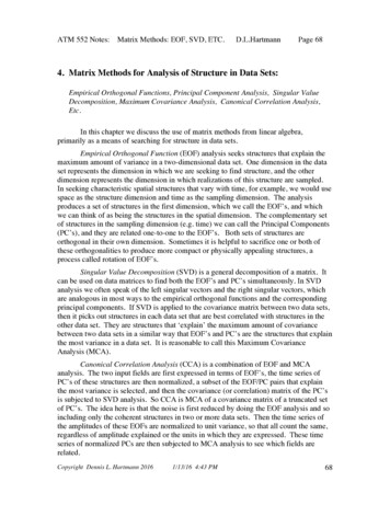
ATM 552 Notes: Matrix Methods: EOF, SVD, ETC.D.L.HartmannPage 73EOF’s and PC’s in ForecastingSuppose we wish to predict y given x1, x2, x3, .xM, but we know that the xi’s areprobably correlated with each other. It is possible and desirable to first determine somenew predictors zi, which are linear combinations of the xi.z1 e11 x1 e12 x 2 e13x3 . e1M x Mz2 e21x1 e22 x2 e23x3 . e2M x M. . .zM eM1x1 eM2 x 2 eM3x3 . eM M xM(4.3)that is, zi eij xj. The matrix of coefficients eij rotates the original set of variables into asecond set.It is possible to determine the eij in such a way that:1) z1 explains the maximum possible amount of the variance of the x’s; z2 explainsthe maximum possible amount of the remaining variance of the x’s; and so forth forthe remaining z’s. No variance is shared between the predictors, so you just sum up thevariance explained by each z. The eij are the set of empirical orthogonal functions, andwhen we project the data xj onto the EOF’s we obtain the principal components, zi,which are the expression of the original data in the new coordinate system. The EOF’sare spatially orthonormal, that is 1, for i jeki eij 0, for i jwhere I is the identity matrix.orET E I(4.4)2) The z’s are orthogonal, linearly independent, or uncorrelated, over the sample.That iszik zkj 0 for i j .(4.5)where the overbar indicates an average over the sample or summing over the k index,which in many applications will be an average over time. This property oforthogonality or lack of correlation in time makes the principal components veryefficient for statistical forecasting, since no variance is shared between the predictorsand the minimum useful correlation is any nonzero one.4.3EOFs Derived as Efficient Representations of Data SetsFollowing Kutzbach (1967), we can show how the mathematical development ofempirical orthogonal functions (EOFs) follows from the desire to find a basis set thatCopyright Dennis L. Hartmann 20161/13/16 4:43 PM73

ATM 552 Notes: Matrix Methods: EOF, SVD, ETC.D.L.HartmannPage 74explains as much as possible of the variance of a data set with the fewest possiblecoordinate directions (unit vectors). This will illustrate that the structure functions wewant are the eigenvectors of the covariance matrix. Suppose we have an observationvector xm, of length M, so that it requires M components to describe the state of thesystem in question. It can also be termed the state vector. If we have N observations ofthe state vector xm then we can think of an observation matrix X xnm , whose n columnsrepresent the n observation times and whose m rows represent the m components of thestate vector. We want to determine a vector e, which has the highest possibleresemblance to the ensemble of state vectors. The projection of this unknown vector ontothe ensemble of data is measured by the inner product of the vector e with the observationmatrix X. To produce an estimate of the resemblance of e to the data that is unbiased bythe size of the data set, we must divide by N. To make the measure of resemblanceindependent of the length of the vector and dependent only on its direction, we shoulddivide by the length of the vector e. The measure of the resemblance of e to the ensembleof data derived by this line of reasoning is,(eT X)2( )( ) 1 1N 1 eT e e T XXT e N 1 eT e(4.6)This is equivalent to maximizing,eT C e ; subject to e T e 1(4.7)C XX T N 1(4.8)and where,is the covariance matrix of the observations (C is really only equal to the usual definitionof the covariance matrix if we have removed the mean value from our data). The lengthof the unknown vector e is constrained to be equal to one so that only the direction of itcan affect its projection on the data set. Otherwise the projection could be madearbitrarily large simply by increasing the length of e.To facilitate a solution to (4.7), suppose that we assume the maximum value of thesquared projection we are looking for is λ. It is equal to the variance explained by thevector e.eT C e λ(4.9)(4.9) corresponds to the classic eigenvalue problem,C e e λor{C λ I} e 0(4.10)This can only be true if,C λ I 0Copyright Dennis L. Hartmann 20161/13/16 4:43 PM(4.11)74

ATM 552 Notes: Matrix Methods: EOF, SVD, ETC.D.L.HartmannPage 75Thus λ is an eigenvalue of the covariance matrix C. The eigenvalues of a real symmetricmatrix are positive, as we expected our λ’s to be when we defined them with (4.9). Ingeneral there will be M of these eigenvalues, as many as there are elements of the statevector x unless the matrix is degenerate (in which case there are only r nonzeroeigenvalues, where r is the rank of the matrix). From (4.9) we can see that each of theseλj is equal to the variance explained by the corresponding ej. To find the empiricalorthogonal function, ej, we can use any number of standard techniques to solve thesystem,(C λ I) e 0j(4.12)jwhich is equivalent to the standard linear algebra problem of diagonalizing the matrix R.It is easy to show that the eigenvectors, ej, are orthogonal. Suppose we have twoeigenvectors ej and ek. From (4.3) we know that,C ej λ j ejC ek λk ek(a)(4.13)(b)Multiply (4.13a) by ekT and transpose the equation. Multiply (4.13b) by ejT. Subtractingthe resulting equations from each other yields,()eTj CT ek eTj C ek λ j λk eTj ek(4.14)Since the covariance matrix C is symmetric, the left-hand side of (4.14) is zero and wehave,e Tj ek 0unlessλ j λk(4.15)Therefore the eigenvectors are orthogonal if the eigenvalues are distinct.We have defined a new basis in the orthonormal eigenvectors ei that can be used todescribe the data set. These eigenvectors are called the empirical orthogonal functions;empirical because they are derived from data; orthogonal because they are so.4.4 Manipulation of EOFs and PCsOriginal Space to EOF Space and back again.It is convenient to order the eigenvalues and eigenvectors in order of decreasingmagnitude of the eigenvalue. The first eigenvector thus has the largest λ and explains thelargest amount of variance in the data set used to construct the covariance matrix. Weneed to know how to find the loading vectors that will allow us to express a particularCopyright Dennis L. Hartmann 20161/13/16 4:43 PM75

ATM 552 Notes: Matrix Methods: EOF, SVD, ETC.D.L.HartmannPage 76state in this new basis. Begin by expanding the equation for the eigenvalues to includeall the possible eigenvalues. The equation (4.9) becomes,ET C E ΛorET XX T E Λ N(4.16)Where E is the matrix whose columns are the eigenvectors ei and L is a square matrixwith the M eigenvalues down the diagonal and all other elements zero. If C is MxM andhas M linearly independent eigenvectors, then the standard diagonalization (4.16) isalways possible.If we defineZ ET X(4.17)Then it follows that,X EZ ,sinceE ET I(4.18)where I is the identity matrix. Equation (4.18) shows how to express the original data interms of the eigenvectors, when the coefficient matrix Z is defined by (4.17). Z containsthe principal component vectors, the amplitudes by which you multiply the EOFs to getthe original data back. One can go back and forth from the original state vector in theoriginal components to the new representation in the new coordinate system by using theeigenvector matrix, as indicated by the transform pair in (4.17) and 4.18). An individualobservation vector xn Xin can thus be expressed asMx n Xin Eij Z jn(4.19)j 1Copyright Dennis L. Hartmann 20161/13/16 4:43 PM76

ATM 552 Notes: Matrix Methods: EOF, SVD, ETC.D.L.HartmannPage 77Projections 101:Suppose we have a set of orthogonal and normalized eigenvectors. The first one mightlook like the following: e11 e 21 e 31 Putting all the eigenvectors into the columns of a square matrix, gives me E, . e M 1 whichhas the following orthonormality property.where I is the identity matrix.ET E IIf I want to PROJECT a single eigenvector onto the data and get an amplitude of thiseigenvector at each time, I do the following, eTX x11 x 21[e11 e 21 e 31 . . . eM 1] x 31 . x M1x12x 22x 32.xM 2x13x23x33.xM 3. x1N . x 2N . x 3N [ z11 z12 . . . x MN z13 . z1N ]where, for example, z11 e11 x11 e21 x21 e 31x 31 . eM1 x M1 . If we do the same forall the other eigenvectors, we will get time series of length n for each EOF, which we callthe principle component (PC) time series for each EOF, Z, which is an NxM matrix.ET X ZCopyright Dennis L. Hartmann 20161/13/16 4:43 PM77

ATM 552 Notes: Matrix Methods: EOF, SVD, ETC.D.L.HartmannPage 78Orthogonality of the Principal Component Time Series.The matrix Z is the coefficient matrix of the expansion of the data in terms of theeigenvectors, and these numbers are called the principal components. The columnvectors of the matrix are the coefficient vectors of length M for the N observationtimes(or cases). Substituting (4.18) into (4.16) we obtain,ET XXT E ET EZZT ET E ZZT Λ NZ ZT Λ Nor1ZZT ΛN(4.20)Thus not only the eigenvectors, but also the PCs are orthogonal. If you like, the Nrealizations expressed in principal component space for any two eigenvectors and theirassociated PCs are uncorrelated in time. The basis set in principal component space, theei’s, is an orthogonal basis set, both in the ‘spatial’ dimension M and the ‘temporal’dimension N.Note that the fraction of the total variance explained by a particular eigenvector is equalto the ratio of that eigenvalue to the trace of the eigenvalue matrix, which is equal to thetrace of the covariance matrix. Therefore the fraction of the variance explained by thefirst k of the M eigenvectors is,kλi i 1Vk M λi(4.21)i 1No other linear combination of k predictors can explain a larger fraction of the variancethan the first k principal components. In most applications where principal componentanalysis is useful, a large fraction of the total variance is accounted for with a relativelysmall number of eigenvectors. This relatively efficient representation of the variance andthe fact that the eigenfunctions are orthogonal, makes principal component analysis animportant part of statistical forecasting.To this point we have assumed that the matrix C is a covariance matrix and that the λ’scorresponded to partial variances. In many applications, however, it is desirable tonormalize the variables before beginning so that C is in fact a correlation matrix and theλ’s are squared correlation coefficients, or fractions of explained variance. The decisionto standardize variables and work with the correlation matrix or, alternatively, to use thecovariance matrix depends upon the circumstances. If the components of the state vectorare measured in different units (e.g., weight, height, and GPA) then it is mandatory to usestandardized variables. If you are working with the same variable at different points(e.g., a geopotential map), then it may be desirable to retain a variance weighting byusing unstandardized variables. The results obtained will be different. In the case of theCopyright Dennis L. Hartmann 20161/13/16 4:43 PM78

ATM 552 Notes: Matrix Methods: EOF, SVD, ETC.D.L.HartmannPage 79covariance matrix formulation, the elements of the state vector with larger variances willbe weighted more heavily. With the correlation matrix, all elements receive the sameweight and only the structure and not the amplitude will influence the principalcomponents.4.5EOF Analysis via Singular Vector Decomposition of the Data MatrixIf we take the two-dimensional data matrix of structure (e.g. space) versussampling (e.g. time) dimension, and do direct singular value decomposition of thismatrix, we recover the EOFs, eigenvalues, and normalized PC’s directly in one step. Ifthe data set is relatively small, this may be easier than computing the dispersion matricesand doing the eigenanalysis of them. If the sample size is large, it may becomputationally more efficient to use the eigenvalue method. Remember first ourdefinition of SVD of a matrix:Singular Value Decomposition: Any m by n matrix X can be factored intoX U Σ VT(4.22)where U and V are orthogonal and Σ is diagonal. The columns of U (m by m) are theeigenvectors of XXT, and the columns of V (n by n) are the eigenvectors of XTX. The rsingular values on the diagonal of Σ (m by n) are the square roots of the nonzeroeigenvalues of both XXT and XTX. .So we suppose that the data matrix X is MxN, where M is the space or structuredimension and N is the time or sampling dimension. More generally, we could think ofthe dimensions as the structure dimension M and the sampling dimension N, but forconcreteness and brevity let’s call them space and time. Now XX T is the dispersionmatrix obtained by taking an inner product over time leaving the covariance betweenspatial points. Thus the eigenvectors of XX T are the spatial eigenvectors, and appear asthe columns of U in the SVD. Conversely, X T X is the dispersion matrix where the innerproduct is taken over space and it represents the covariance in time obtained by usingspace as the sampling dimension. So the columns of V are the normalized principalcomponents that are associated uniquely with each EOF. The columns of U and V arelinked by the singular values, which are down the diagonal of Σ. These eigenvaluesrepresent the amplitude explained, however, and not the variance explained, and so arethe proportional to the square roots of the eigenvalues that would be obtained byeigenanalysis of the dispersion matrices. The eigenvectors and PC’s will have the samestructure, regardless of which method is used, however, so long as both are normalized tounit length.Copyright Dennis L. Hartmann 20161/13/16 4:43 PM79

ATM 552 Notes: Matrix Methods: EOF, SVD, ETC.D.L.HartmannPage 80To illustrate the relationship between the singular values of SVD of the data matrixand the eigenvalues of the covariance matrix, consider the following manipulations.Let’s assume that we have modified the data matrix X to remove the sample mean fromevery element of the state vector, so that X X X . The covariance matrix is given byC XXT / n(4.23)and the eigenvectors and eigenvectors are defined by the diagonalization of C.C EΛET(4.24)TNow if we take the SVD of the data matrix, X UΣV , and use it to compute thecovariance matrix, we get:C UΣV T (UΣV T )T / n UΣV T VΣ T UT / n(4.25) UΣΣ T UT / nFrom this we infer that: U E, Λ ΣΣT / n or λ i σ i 2 / n , so there is a peskyfactor of n, the sample size, between the eigenvalues of the covariance matrix, and thesingular values of the original data matrix.Also, from EOF/PC analysis we noted that the principal component time series areobtained from Z ET X , if we apply this to the singular value decomposition of X, weget (see 4.17-4.18),Z ET X ET UΣVT ET EΣVT ΣVTZ ΣVT(4.26)Notice that as far as the mathematics is concerned, both dimensions of the data setare equivalent. You must choose which dimension of the data matrix contains interestingstructure, and which contains sampling variability. In practice, sometimes only onedimension has meaningful structure, and the other is noise. At other times both can havemeaningful structure, as with wavelike phenomena, and sometimes there is nomeaningful structure in either dimension.Note that in the eigenanalysis,ZZT ET XXT E ETCEN ΛN ,(4.27)whereas in the SVD representation,ZZT ΣVT VΣ T ΣΣ T ,Copyright Dennis L. Hartmann 20161/13/16 4:43 PM(4.28)80

ATM 552 Notes: Matrix Methods: EOF, SVD, ETC.D.L.HartmannPage 81so we must have thatΣΣ T ΛN , or σ k2 λk N .4.6(4.29)Presentation of EOF Analysis ResultsAfter completing EOF analysis of a data set, we have a set of eigenvectors, orstructure functions, which are ordered according to the amount of variance of the originaldata set that they explain. In addition, we have the principal components, which are theamplitudes of these structure functions at each sampling time. Normally, we onlyconcern ourselves with the first few EOFs, since they are the ones that explain the mostvariance and are most likely to be scientifically meaningful. The manner in which theseare displayed depends on the application at hand. If the EOFs represent spatial structure,then it is logical to map them in the spatial domain as line plots or contour plots, possiblyin a map projection that shows their relation to geographical features.One can plot the EOFs directly in their normalized form, but it is often desirableto present them in a way that indicates how much real amplitude they represent. Oneway to represent their amplitude is to take the time series of principal components for thespatial structure (EOF) of interest, normalize this time series to unit variance, and thenregress it against the original data set. This produces a map with the sign anddimensional amplitude of the field of interest that is explained by the EOF in question.The map has the shape of the EOF, but the amplitude actually corresponds to theamplitude in the real data with which this structure is associated. Thus we get structureand amplitude information in a single plot. If we have other variables, we can regressthem all on the PC of one EOF and show the structure of several variables with thecorrect amplitude relationship, for example, SST and surface vector wind fields can bothbe regressed on PCs of SST.How to scale and plot EOF’s and PC’s:Let’s suppose we have done EOF/PC analysis using either the SVD of the data (describedin Section 4.5), or the eigenanalysis of the covariance matrix. We next want to plot theEOF’s to show the spatial structure in the data. We would like to combine the spatialstructure and some amplitude information in a single plot. One way to do this is to plotthe eigenvectors, which are unit vectors, but to scale them to the amplitude in the data setthat they represent.Let’s Review:SVD of Data Matrix Approach:Copyright Dennis L. Hartmann 20161/13/16 4:43 PM81

ATM 552 Notes: Matrix Methods: EOF, SVD, ETC.D.L.HartmannPage 82Before we look at the mathematics of how to do these regressions, let’s first review theSVD method of computing the EOFs and PCs.We start with a data matrix X, with n columns and m rows (nxm), and SVD it, giving thefollowing representation.X UΣVT(4.30)the columns of U are the column space of the matrix, and these correspond to theeigenvectors of EOF analysis. The columns of V are the unit vectors pointing in thesame direction and the PC’s of EOF analysis. They are the normalized time variability ofthe amplitudes of the EOFs, the normalized PCs. The diagonal elements of Σ, are theamplitudes corresponding to each EOF/PC pair.Eigenanalysis of Covariance Matrix:If we take the product across the sampling dimension of the original data matrix X, weget the

and N times, you can make the spatial structure into a big vector LxK M long, and then analyze the resulting (LxK)xN MxN data matrix. (A vector is a matrix where one dimension is of length 1, e.g. an 1xN matrix is a vector). So we can visualize a two-dimensional data matrix X as follows: N X M Xi,jwherei 1,M;j 1,N