Transcription
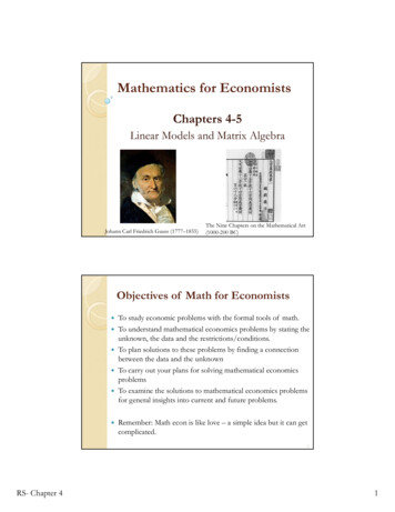
Mathematics for EconomistsChapters 4-5Linear Models and Matrix AlgebraJohann Carl Friedrich Gauss (1777–1855)The Nine Chapters on the Mathematical Art(1000-200 BC)Objectives of Math for Economists To study economic problems with the formal tools of math.To understand mathematical economics problems by stating theunknown, the data and the restrictions/conditions.To plan solutions to these problems by finding a connectionbetween the data and the unknownTo carry out your plans for solving mathematical economicsproblemsTo examine the solutions to mathematical economics problemsfor general insights into current and future problems.Remember: Math econ is like love – a simple idea but it can getcomplicated.2RS- Chapter 41
4. Linear AlgebraSome early history: The beginnings of matrices and determinants goes back to thesecond century BC although traces can be seen back to the fourthcentury BC. But, the ideas did not make it to mainstream mathuntil the late 16th century The Babylonians around 300 BC studied problems which lead tosimultaneous linear equations. The Chinese, between 200 BC and 100 BC, came much closer tomatrices than the Babylonians. Indeed, the text Nine Chapters on theMathematical Art written during the Han Dynasty gives the firstknown example of matrix methods. In Europe, 2x2 determinants were considered by Cardano at theend of the 16th century and larger ones by Leibniz and, in Japan, bySeki about 100 years later. 4. What is a Matrix? A matrix is a set of elements, organized into rows and columnsrowscolumns a c b d a and d are the diagonal elements. b and c are the off-diagonal elements. Matrices are like plain numbers in many ways:they can be added, subtracted, and, in somecases, multiplied and inverted (divided).Arthur Cayley (1821 – 1895, England)RS- Chapter 42
4. Matrix: Details Examples: aA 11 a 12a 21 ;a 22 b b1b2b3 Dimensions of a matrix: numbers of rows by numbers ofcolumns. The Matrix A is a 2x2 matrix, b is a 1x3 matrix. A matrix with only 1 column or only 1 row is called a vector. If a matrix has an equal numbers of rows and columns, it iscalled a square matrix. Matrix A, above, is a square matrix. Usual Notation:Upper case lettersLower case matrices vectors54. Matrix: DetailsIn econometrics, we have data, say T (or N) observations, on adependent variable, Y, and on k explanatory variables, X. Under the usual notation, vectors will be column vectors: y andxk are Tx1 vectors: &xj j 1,., k X is a Txk matrix:X Its columns are the k Tx1 vectors xj. It is common to treat x1 asvector of ones, ί. 6RS- Chapter 43
4.1 Special Matrices: Identity and Null 1 0 0 0 1 0 0 0 1 0 0 0 0 0 0 0 0 0 Identity Matrix: A square matrix with 1’s alongthe diagonal and 0’s everywhere else. Similar toscalar “1.” Null matrix: A matrix in which all elements are0’s. Similar to scalar “0.” Both are diagonal matriceselements are zero. Both are examples of symmetric and idempotent matrices. As we willsee later:- Symmetric: A AT- Idempotent: A A2 A3 7 off-diagonal4.1 Matrix: Elementary Row Operations Elementary row operations:- Switching: Swap the positions of two rows- Multiplication: Multiply a row by a non-zero scalar- Addition: Add to one row a scalar multiple of another. An elementary matrix is a matrix which differs from the identitymatrix by one single elementary row operation. If the matrix subject to elementary row operations is associatedto a system of linear equations, then these operations do notchange the solution set. Row operations can make the problemeasier. Elementary row operations are used in Gaussian elimination toreduce a matrix to row echelon form.RS- Chapter 484
4.1 Matrix multiplication: Details Multiplication of matrices requires a conformability conditionThe conformability condition for multiplication is that thecolumn dimensions of the lead matrix A must be equal to therow dimension of the lag matrix B.If A is an (mxn) and B an (nxp) matrix (A has the same numberof columns as B has rows), then we define theproduct of AB.nAB is (mxp) matrix with its ij-th element is j 1 aijbjkWhat are the dimensions of the vector, matrix, and result? b11aB a11 a12 b21b1222b13 c c11b23 c12c13 a11b11 a12b21 a11b12 a12b22 a11b13 a12b23 Dimensions: a(1x2), B(2x3) c(1x3)94.1 Transpose Matrix The transpose of a matrix A is another matrix AT (also writtenA′) created by any one of the following equivalent actions:- write the rows (columns) of A as the columns (rows) of AT- reflect A by its main diagonal to obtain ATFormally, the (i,j) element of AT is the (j,i) element of A:[AT]ij [A]jiIf A is a m n matrix AT is a n m matrix.(A')' AConformability changes unless the matrix is square. 3 1 3 8 9 Example : A A 8 0 104 9 4 10RS- Chapter 45
4.1 Transpose Matrix: Example – X’ In econometrics, an important matrix is X’X. Recall X:X a (Txk) matrix a (kxT) matrixThen,X’114.1 Basic Operations Addition, Subtraction, Multiplication a b e f a e b f c d g h c g d h Just add elements a b e f a e b f c d g h c g d h Just subtract elementsf ae bg h ce dgMultiply each row byeach column and add a b e c d g a b ka kb k kc kd cd af bh cf dh Multiply eachelement by the scalar12RS- Chapter 46
4.1 Basic Matrix Operations: Examples Matrix addition Matrix subtraction Matrix multiplication Scalar multiplication 2 1 3 1 5 2 7 9 0 2 7 11 A2 x 2 B2 x 2 C2 x 2 2 1 1 0 1 1 7 9 2 3 5 6 2 1 1 0 4 3 7 9 x 2 3 26 27 A 2 x 2 xB2 x 2 C 2 x 21 2 4 1 4 1 2 8 6 1 3 413 1 8 134.1 Basic Matrix Operations: X′X A special matrix in econometrics, X′X (a kxk matrix): & X’ Recall X (Txk): X in 1 xi21 in 1 xi1 xi 2 n x x in 1 xi22X'X i 1 i 2 i1 . nn i 1 xiK xi1 i 1 xiK xi 2 xi1 x in 1 i 2 xi1 xi 2 . . xik in 1x i x iRS- Chapter 4 xi21. in 1 xi1 xiK . in 1 xi 2 xiK n xi 2 xi1 i 1 . . in 1 xiK2 xiK xi1xi1 xi 22i2x.xiK xi 2 xi1 xiK . xi 2 xiK . . xiK2 .xiK 147
4.1 Basic Matrix Operations: ί′X Recall ί is a column vector of ones (in this case, a Tx1 vector):11ί 1Given X (Txk), then ί’ X is a 1xk vector: ί’X1 1 Note: If x1 is a vector of ones (representing a constant in thelinear classical model), then: 1 T(“dot product”)ί’ x1 154.1 Basic Matrix Operations: R Many ways to create a vector (c, 2:7, seq, rep, etc) or a matrix (c,cbind, rbind). Usually, matrices will be data –i.e., read as inpu: v - c(1, 3, 5) v[1] 1 3 5 A - matrix(c(1, 2, 3, 7, 8, 9), ncol 3) A[,1] [,2] [,3][1,]138[2,]279 B - matrix(c(1, 3, 1, 1, 2, 0), nrow 3) B[,1] [,2]RS- Chapter 4[1,]11[2,]32[3,]1016168
4.1 Basic Matrix Operations: R Matrix addition/substraction: /- --element by element Matrix multiplication: %*% C - A%*%B#A is 2x3; B is 3x2 C[,1] [,2][1,] 187[2,] 32 16 Scalar multiplication: * --elementwise multiplication of twomatrices/vectors 2*C[,1] [,2][1,] 36 1417[2,] 64 32174.1 Basic Matrix Operations: R Matrix transpose: t t(B)#B is 3x2; t(B) is 2x3[,1] [,2] [,3][1,]131[2,]120 X'X t(B)%*%B# command crossprod(B) is more efficient[,1] [,2][1,] 117[2,]5 7dot product i - c(1,1,1); t(i)%*%v[,1][1,]RS- Chapter 49# v - c(1, 3, 5)18189
4.1 Laws of Matrix Addition & Multiplication Commutative law of Matrix Addition: A B B Aa b b a bb a aA B 11 12 11 12 11 11 12 12 a21 a22 b21 b22 a21 a21 b22 a22 b a b b a a b aB A 11 12 11 12 11 11 12 12 b21 b22 b21 b22 b21 a21 b22 a22 Matrix Multiplication is distributive across Additions:A (B C) AB AC(assuming comformability applies).194.1 Matrix Multiplication Matrix multiplication is generally not commutative. That is,AB BA even if BA is conformable(because different dot product of rows or col. of A&B) 1 2 0 1 A ,B 6 7 3 4 1 0 2 6 1 1 2 7 12AB 3 0 4 6 3 1 4 7 2413 25 0 1 1 3 0 2 1 4 3 4 BA 6 2 7 4 27 40 6 1 7 3 20RS- Chapter 410
4.1 Matrix multiplication Exceptions to non-commutative law:AB BA iffB a scalar,B identity matrix I, orB the inverse of A -i.e., A-1 Theorem: It is not true that AB AC B CProof: 1A 1 120 21 1 1 ; B 0 1 3 1111 2 0 ; C 1 20 1 13Note: If AB AC for all matrices A, then B C.2 1 1 214.1 Inverse of a Matrix Identity matrix: AI A 1 0 0 I 3 0 1 0 0 0 1 Notation: Ij is a jxj identity matrix.Given A (mxn), the matrix B (nxm) is a right-inverse for A iffAB Im Given A (mxn), the matrix C (mxn) is a left-inverse for A iffCA In 22RS- Chapter 411
4.1 Inverse of a Matrix Theorem: If A (mxn), has both a right-inverse B and a left-inverse C,thenC B.Proof:We haveAB Im and CA In.Thus,and C(AB) (CA)B InB BC(AB) C Im C C(nxm) B(mxn)Note:- This matrix is unique. (Suppose there is another left-inverse D,then D B by the theorem, so D C.).- If A has both a right and a left inverse, it is a square matrix. Itis usually called invertible. We say “the matrix A is non-singular.”4.1 Inverse of a MatrixRS- Chapter 4 Inversion is tricky:(ABC)-1 C-1B-1A-1 Theorem: If A (mxn) and B (nxp) have inverses, then AB isinvertible and (AB)-1 B-1A-1Proof:We haveAA-1 Im and A-1A InBB-1 In and B-1B IpThus,B-1A-1(AB) B-1 (A-1A) B B-1 InB B-1 B Ip(AB) B-1A-1 A (BB-1) A-1 A In A-1 A A-1 Im AB is invertible and (AB)-1 B-1A-1 More on this topic later.2412
4.1 Transpose and Inverse Matrix (A B)' A' B'If A' A, then A is called a symmetric matrix.Theorems:- Given two comformable matrices A and B, then (AB)' B'A'- If A is invertible, then (A-1)' (A')-1 (and A' is also invertible).254.1 Partitioned MatrixA partitioned matrix is a matrix which has been broken intosections called blocks or submatrices by horizontal and/or verticallines extending along entire rows or columns. For example, the3xm matrix can be partitioned as: a11a 21a12 a 22 a31 a32 a1m a2 m A11 (2x 2) A21 (1x 2) a3 m A12 (2x(m 2)) A22 (1x( m 2)) Augmented matrices are also partitioned matrices. They havebeen partitioned vertically into two blocks. Partitioned matrices are used to simplify the computation ofinverses. RS- Chapter 42613
4.1 Partitioned MatrixIf two matrices, A and B, are partitioned the same way, additioncan be done by blocks. Similarly, if both matrices are comformablepartitioned, then multiplication can be done by blocks. A block diagonal matrix is a partitioned square matrix, with maindiagonal blocks square matrices and the off-diagonal blocks arenull matrices. Nice Property: The inverse of a block diagonal matrix is just theinverse of each block. A100 A2 0 0 0 0 An A1 10 0 0A2 1 0 0 0 An 1 274.1 Partitioned Matrix: Partitioned OLS Solution In the Classical Linear Model, we have the OLS solution: 1b (X ' X ) X ' y b X ' X 1 1 1 b2 X 2 ' X 1 1X1 ' X 2 X1 ' y X 2 ' X 2 X 2 ' y Use of the partitioned inverse result produces a fundamentalresult, the Frisch-Waugh (1933) Theorem: To calculate b2 (or b1)we do not need to invert the whole matrix. For this result, we needthe southeast element in the inverse of (X′X)-1: [ ]-1(2,1) X 1 'X 1 X 2 'X 1X 1 'X 2 X 2 'X 2 -1[ ]-1(2,2)With the partitioned inverse, we get:b2 [ ]-1(2,1) X1′y [ ]-1(2,2) X2′y28RS- Chapter 414
4.1 Partitioned Matrix: Partitioned OLS Solution From partitioned inverse: As we will derive later:b2 [ ]-1(2,1) X1′y [ ]-1(2,2) X2′y X ' X X1 ' X 2 1. Matrix X'X 1 1 X 2 ' X1 X 2 ' X 2 ( X ' X ) 1 ( X1 ' X1 ) 1 X1 ' X 2 DX 2 ' X1 ( X1 ' X1 ) 1 ( X1 ' X1 ) 1 X1 ' X 2 D 2. Inverse 1 1 DX 2 ' X1 ( X1 ' X1 ) 1D where D [ X 2 ' X 2 X 2 ' X1 ( X1 ' X1 ) 1 X1 ' X 2 ] 1 [ X 2 ' (I X1 ( X1 ' X1 ) 1 X1 )' X 2 ] 1 D [ X 2 ' M1 X 2 ] 1 [ ]-1(2,1) -D X2’X1(X1’X1)-1[ ]-1(2,2) D [X2’M1X2]-1b2 [ ]-1(2,1) X1′y [ ]-1(2,2) X2′y [X2′M1X2]-1X2′M1yThe algebraic result is:4.1 Properties of Symmetric Matrices Definition:If A' A, then A is called a symmetric matrix. Theorems:- If A and B are nxn symmetric matrices, then (AB)' BA- If A and B are nxn symmetric matrices, then (A B)' B A- If C is any nxn matrix, then B C'C is symmetric. Useful symmetric matrices:V X’XP X(X’X)-1X’M I – P I - X(X’X)-1X’P: Projection matrixM: Residual maker30RS- Chapter 415
4.1 Application 1: Linear System There is a functional form relating a dependent variable, y, and kexplanatory variables, X. The functional form is linear, but itdepends on k unknown parameters, . The relation between y andX is not exact. There is an error, . We have T observations of yand X. Then, the data is generated according to:i 1, 2, ., T.yi Σj 1,.k xk,i k iOr using matrix notation:y X where y & are (Tx1); X is (Txk); and is (kx1). We will call this relation data generating process (DGP). The goal of econometrics is to estimate the unknown vector .314.1 Application 2: System of Equations Assume an economic model as system of linear equations with:where i 1,., m rows, j 1,., n columnsaij parameters,xi endogenous variables (n),di exogenous variables and constants (m).a11 x1 a12 x2 . a1n xn d1a21 x1 a22 x2 . a2n xn d2.am1 x1 am2 x2 . amn xn dm We can write this system using linear algebra notation: A x d d column vectorA (mxn) matrix RS- Chapter 4x column vectorQ: What is the nature of the set of solutions to this system?3216
4.1 Application 2: System of EquationsSystem of linear equations:Ax dwhereA (mxn) matrix of parametersx column vector of endogenous variables (nx1)d column vector of exogenous variables and constants (mx1) Solve for x*Questions:- For what combinations of A and d there will zero, one, many oran infinite number of solutions?- How do we compute (characterize) those sets of solutions? 334.1 Solution of a General Equation System Theorem: Given A (mxn). If A has a right-inverse, then theequation Ax d has at least one solution for every d (mx1).Proof:Pick an arbitrary d. Let H be a right-inverse (so AH Im).Define x* Hd.Thus,Ax* A Hd Imd d x* is a solution. 34RS- Chapter 417
4.1 Solution of a General Equation System Theorem: Given A (mxn). If A has a left-inverse, then theequation Ax d has at most one solution for every d (mx1). Thatis, if Ax d has a solution x* for a particular d, then x* is unique.Proof:Suppose x* is a solution and z* is another solution. Thus, Ax* dand Az* d. Let G be a left-inverse for A (so GA In).Ax* d GA x* Gd Inx* x* Gd.Az* d GA z* Gd Inz* z* Gd.Thus,x* z* Gd. 354.1 Solution of a General Equation System Problem with the previous proof ? We’re assuming the leftinverse exists (and there’s always a solution).Assume the 2x2 model2x y 124x 2y 24 Find x*, y*:y 12 – 2x4x 2(12 – 2x) 244x 24 – 4x 240 0 ? indeterminante!Why?4x 2y 242(2x y) 2(12) one equation with twounknowns2x y 12 Conclusion: Not all simultaneousequation models have solutions(not all matrices have inverses).36RS- Chapter 418
4.1 Solution of a General Equation System Theorem: Given A (mxn) invertible. Then, the equation Ax dhas one and only one solution for every d (mx1).Proof:Trivial from previous two theorems. Given an invertible matrix, A, use the “solve” command: A[,1] [,2][1,] 187[2,] 32 16 d - c(2, 1) x - solve(A, d) x[1] 0.390625 -0.718750374.1 Linear dependence and Rank: ExampleA set of vectors is linearly dependent if any one of them can beexpressed as a linear combination of the remaining vectors;otherwise, it is linearly independent. Formal definition: Linear independence (LI)The set {u1,.,uk} is called a linearly independent set of vectors iffc1 u1 . ckuk θ c1 c2 . ck, 0. Notes:- Dependence prevents solving a system of equations. Moreunknowns than independent equations.- The number of linearly independent rows or columns in a matrixis the rank of a matrix (rank(A)). 38RS- Chapter 419
4.1 Linear dependence and Rank: Example Examples:v1' 5 12 v2' 10 24 5 10 v1' A ' 12 24 v2 2v1/ v2/ 0 / rank ( A) 1 2 1 4 v1 ; v 2 ; v3 ; 7 8 5 3v1 2v 2 6 2 1 4 A 7 8 5 21 2 16 4 5 v33v1 2v 2 v3 0 rank ( A) 2394.2 Application 1: One Commodity MarketModel (2x2 matrix)Economic Model1) Qd a – bP (a,b 0)2) Qs -c dP (c,d 0)3) Qd Qs Find P* and Q* Scalar Algebra form(Endogenous Vars ::4) 1Q bP aa cb dad bcQ* b dP* Constants)5) 1Q – dP -c40RS- Chapter 420
4.2 Application 1: One Commodity MarketModel (2x2 matrix)Matrix algebrab Q 1 a 1 d P c Ax d Q * 1 * 1 P x * A 1 db d 1 a c 414.2 Application 2: Finite Markov Chains Markov processes are used to measure movements over time.Employees at time 0 are distributed over two plants A & Bx 0/ A0B0 100 100 The employeesstay and move between each plants w/ a known probabilityPAB .7 .3 PM AA PBA PBB .4 .6 At the end of one year, how many employees will be at each plant? A1PAB PB0 AA A0 PAA A0 PBA B0 PAB B0 PBB P BA PBB .7 .3 100 100 .3 *100 .6 *100 .7 *100 .4 *100, .4 .6 B1 x 0/ M A0 110 90 42RS- Chapter 421
4.2 Application 2: Finite Markov ChainsAt the end of two years, how many employees will be at each plant?PAB PB0 AA 110 90 PBA PBB PAB PAA PAB P A0 B0 AA P BA PBB PBA PBB A1B1 x 0/ M A0 A2B2 x 0/ M 2 .7 .3 110 90 .7 *110 .4 * 90, .3 *110 .6 * 90 .4 .6 113 87 After k years : AkBk x 0/ M k434.3 Definite Matrices - FormsA form is a polynomial expression in which each componentterm has a uniform degree. A quadratic form has a uniform seconddegree. Examples:9x 3y 2z6x2 2xy 2y2x2z 2yz2 2y3-first degree form.-second degree (quadratic) form.-third degree (cubic) form.A quadratic form can be written as: x’A x, where A is asymmetric matrix. 44RS- Chapter 422
4.3 Definite Matrices - FormsFor one variable, a quadratic form is the familiar: y a x2If a 0, then a x2 is always non-negative, and equals 0 only whenx 0. We call a form like this positive definite.If a 0, then a x2 is always non-positive, and equals 0 only whenx 0. We call a form like this negative definite.There are two intermediate cases, where the form can be equal to0 for some non-zero values of x: negative/positive semidefinite. For a general quadratic form, y x’A x, we say the form isPositive definite if y is invariably positive (y 0)Positive semi-definite if y is invariably non-negative (y 0)Negative semi-definite if y is invariably non-positive (y 0)Negative definite if y is invariably negative (y 0)Indefinite if y changes signs.454.3 Definite Matrices - Definition A quadratic form is said to be indefinite if y changes signs.A symmetric (n n) A is called positive definite (pd), positve semidefinite(psd), negative semidefinite (nsd) and negative definite (nd) according to thecorresponding sign of the quadratic form, y. For example, if y x’A x, is positive, for any non-zero vector x ofn real numbers; we say A is positive definite.Example: Let A X′X.Then, z′A z z′X′X z v′v 0. X′X is pd In general, we use eigenvalues to determine the definiteness of a46matrix (and quadratic form).RS- Chapter 423
4.4 Upper and Lower Triangular MatricesA square (nxn) matrix C is:-Upper Triangular (UT) iff Cij 0 for i j(if the diagonal elements are all equal to 1,we have a upper-unit triangular (UUT) matrix) -Lower Triangular (LT) iff Cij 0 for i j(if the diagonal elements are all equal to 1,we have a lower-unit triangular (LUT) matrix) 1 0 0 0 2 12000125 6 UT1 0 0 LT0 -Diagonal (D) iff Cij 0 for i j Theorems:The product of the two UT (UUT) matrices is UT (UUT).The product of the two LT (LUT) matrices is LT (LUT).The product of the two D matrices is D.474.4 UT & LT Matrices – LU FactorizationAn (nxn) matrix A can be factorized, with proper row and/orcolumn permutations, into two factors, an LT matrix L and an UTmatrix U: l11 0A LU l 21 l 22 l31 l32 u11 u12 x 0 u22 l33 0000u13 u 23 u33 Without permutations in A, the factorization may fail. We havean n2 by n2 system. For example, given a11 l11 u11, if a11 0, then atleast one of l11 & u11 has to be 0, which implies either L or U issingular (impossible if A is non-singular). A proper permutation matrix, P, is enough for LU factorization.It is called LU factorization with Partial Pivoting (or PA 48LU). RS- Chapter 424
4.4 UT & LT Matrices – Forward Substitution The LU decomposition requires 2n3/3 (plus lower order terms)operations or “flops” –i.e., floating point operations ( ,-,x,/).When n is large, n3 dominates, we describe this situation with“order n3”or O(n3). Q: Why are we interested in these matrices?Suppose Ax d, where A is LT (with non-zero diagonal terms).Then, the solutions are recursive (forward substitution).Example:x1 d1/a11a21 x1 a22 x2 d2a31 x1 a32 x2 a33 x3 d3Note: For an nxn matrix A, this process involves n2 flops.49494.4 UT & LT Matrices – Back Substitution Similarly, suppose Ax d, where A is UT (with non-zero diagonalterms). Then, the solutions are recursive (backward substitution).Example:a11 x1 a12 x2 a13 x3 d1a22 x2 a23 x3 d2x3 d3/a31Note: Again, for A(nxn), this process involves n2 flops.50RS- Chapter 425
4.4 UT & LT Matrices – Linear Systems Finding a solution to Ax dGiven A (nxn). Suppose we can decompose A into A LU, where Lis LUT and U is UUT (with non-zero diagonal).ThenAx d LUx d.Suppose L is invertible Ux L-1d c(or d Lc) solve by forward substitution for c.Then, Ux c (Gaussian elimination) solve by backwardsubstitution for x. Theorem:If A (nxn) can be decomposed A LU, where L is LUT and U isUUT (with non-zero diagonal), then Ax d has a unique solution51for every d.4.4 UT & LT Matrices – LDU Decomposition We can write a “symmetric” decomposition. Since U has nonzero diagonal terms, we can write U DU*, where U* is UUT.Example: 2 4 8 2 0 0 1 2 4 U 0 3 6 ; D 0 3 0 ; U * 0 1 2 0 0 5 0 0 5 0 0 1 Theorems:- If we can write A (nxn) as A LDU, where L is LUT, D isdiagonal with non zero diagonal elements, and U is UUT, then L,D, and U are unique.- If we can write A (nxn) as A LDU, and A is symmetric, then wecan write A LDL’.52RS- Chapter 426
4.4 Cholesky Decomposition Theorem: Cholesky decompositionA is a symmetric positive definite matrix (A symmetric, A LDL’,and all diagonal elements of D are positive), then A HH’.Proof:Since A is symmetric, then A LDL’.The product of a LUT matrix and a D matrix is a LUT matrix.Let D* D1/2 and L be a LT matrix.Then H LD* is matrix is LT A HH’. H is called the Cholesky factor of A (‘square root’ of a pd matrix.) The Cholesky decomposition is unique. It is used in thenumerical solution of systems of equations, non-linearoptimization, Kalman filter algorithms, IRF of VARs, etc.534.4 Cholesky decomposition: Algorithm Let’s partition matrices A HH’ as: a11 A21T l11A21 A22 L210 l11 L22 0LT21 l112 LT22 l11 L21 L L L22 L l11 LT21T21 21T22/ Algorithm1. Determine l11 and L21:(if A is pd a11 0)l11 a11 &L21 (1/l11) A212. Compute L22 from A22 L21 L21T L22 L22T(if A is pd A22 L21 L21T A22 A21A21T/a11 is pd)André-Louis Cholesky (1875–1918, France)RS- Chapter 45427
4.4 Cholesky decomposition: Algorithm Example:55554.4 Cholesky decomposition: Algorithm Example:Note: Again, for A(nxn), the Cholesky decomposition involves n3/3flops.56RS- Chapter 428
4.4 Cholesky decomposition: Application System of EquationsIf A is a positive definite matrix, then we can solve Ax d by(1) Compute the Cholesky decomposition A HH′.(2) Solve Hy d for y,(forward solution)(3) With y known, solve H′x y for x.(backward solution)3Q: How many flops? Step (1): n /3 flops, Steps (2) (3): 2n2 flops.Note: A-1 is not computed (Gauss-Jordan methods needs 4n3 flops) Ordinary Least Squares (OLS)Systems of the form Ax d with A symmetric and pd arecommon in economics. For example, the normal equations in OLSproblems are of this form (the unknown is b):(y - Xb)′ X 0 X′X b X′ yNo need to compute (X′X)-1 ( A-1) to solve for b.574.5 Inverse matrix (Again) RS- Chapter 4Review- AA-1 I- A-1A I- Necessary for matrix to be square to have unique inverse.- If an inverse exists for a square matrix, it is unique- (A')-1 (A-1)’- If A is pd, then A-1 H’-1H-1- Solution to A x dA-1A x* A-1 dI x* A-1 d x* A-1 d (solution depends on A-1)- Linear independence a problem to get x*- Determinant test! (coming soon)5829
4.5 Inverse of a Matrix: Calculation Theorem: Let A be an invertible (nxn) matrix. Suppose that asequence of elementary row-operations reduces A to the identitymatrix. Then, the same sequence of elementary row-operationswhen applied to the identity matrix yields A-1. a d gbc 10ef 01hi 00 1 0 00100 r0 u1 xsvy0 0 1 t w z Process: Append the identity matrix to A. Subtract multiples of the otherrows from the first row to reducethe diagonal element to 1. Transform I as you go. When the original A matrixbecomes I, the original identityhas become A-1.4.5 Determination of the Inverse(Gauss-Jordan Elimination)all A, X and I are (nxn)square matricesAX I1) Augmentedmatrix[A I ]X A-12) Transform (using elementary rowoperations) augmented matrix[ UT H]Gauss elimination[ I K]Gauss-Jordaneliminationfurther rowoperationsIX KI X X A-1 K A-1Wilhelm Jordan (1842– 1899, Germany)RS- Chapter 430
4.5 Gauss-Jordan Elimination: Example 1Find A-1 using the Gauss-Jordan method. 2 1 1 A 1 2 1 1 1 2 Process: Expand A I. Start scaling and adding rows to get I A-1.1.2. 2 1 1 1 0 0 1 R1 (1 / 2 )A I 1 2 1 0 1 0 1 1 1 1 2 0 0 1 1 1 1 122121120120122121120120 10 0 21 ( 1) & R31 ( 1) 01 0 R 0 1 0 123212121232 0 0 1 0 0 1 0 0 1 0 0 1 121 21 24.5 Gauss-Jordan Elimination: Example 13.4.5.RS- Chapter 4 1 0 0 123212121232121 21 2 1 0 0 12121332121 31 2121343121 31 3 1 0 0 1121210 0 0 1 2 ( 2 / 3)1 0 R A 0 00 1 02300231 312121332112 0 1 32 ( 1 / 2 )0 R 0 01 12 0 1 3 (3 / 4)0 R 0 01 121010121 31 2121343121 31 31213121 31 4102300231 30231 4 0 0 1 0 0 1 0 0 3 4 Gausselimination31
4.5 Gauss-Jordan Elimination: Example 16.7. 1 0 0 1201 1 0 0 120100111213121 31 4231 458 14 141834 14 0 1 23 ( 1 / 3 ) & R13 ( 1 / 2 ) 00 R 3 0 4 1201001 3 1 0 08 1 R12 ( 1 / 2 ) 0 1 04 3 0 0 1 4 68 14 140 1 0 0 8. I A 1 0 1 0 0 0 1 68 14 142834 14 2 3 48 1 1 A 1 4 43 1 44 58 14 142834 14 1434 141834 14 2 8 1 4 3 4 3 8 1 4 3 4 GaussJordanelimination 1 4 1 4 3 4 4.5 Gauss-Jordan Elimination: Example 2Partitioned inverse (using the Gauss-Jordan method).11 XX XY I 0 XX1 R1 I XX0 XY XX 0 I YY YX YY 0 I YX11 I0 XX XY XXR2 YX R12. 1 1 0 YY YX XX XY YX XX I 1.3.11 I XX0 XY XX 1ID( YX XX) D 01[ YY YX XX XY ] 1 R21where D [ YY YX XX XY ] 14.RS- Chapter 411111 I 0 XX XX XY D YX XX XX XY D R1 XX R2 XY 1)D D( YX XX 0 I32
4.5 Gauss-Jordan Elimination: Computations Q: How many flops to invert a matrix with the G-J method?A: Avoid inverses! But, if you must. The process of zeroing outone element of the left-hand matrix requires multiplying the lineto be subtracted by a constant (2n flops), and subtracting it (2nflops). This must be done for (approximately) n2 matrix elements.Thus, the number of flops is about equal to 4n3 by the G-Jmethod. Using a standard PC (100 Gigaflops, 109, per second), for a30x30 matrix, the time required is less than a millisecond,comparing favorably with 1021 years for the method ofcofactors. More sophisticated (optimal) algorithms, taking advantage ofzeros –i.e., the sparseness of the matrix-, can improve to n3 flops.4.5 Matrix inversion: Note It is not possible to divide one matrix by another. That is, wecan not write A/B. For two matrices A and B, the quotient canbe written as AB-1 or B-1A. In general, in matrix algebra AB-1 B-1A.Thus, writing A/B does not clearly identify whether it representsAB-1 or B-1A.We’ll say B-1 post-multiplies A (for AB-1) andB-1 pre-multiplies A (for B-1A) Matrix division is matrix inversion.66RS- Chapter 433
4.5 Matrix inversion: R To find the inverse of a matrix or solve a system of equations,use "solve" A[,1] [,2][1,] 187[2,] 32 16 solve(A)[,1][,2][1,] 0.25 -0.109375[2,] -0.50 0.281250 Solve system Ax d d - c(2, 1) x - solve(A, d); x[1] 0.390625 -0.718750674.6 Trace of a Matrix The trace of an nxn matrix A is defined to be the sum of theelements on the main diagonal of A:trace(A) tr(A) Σi aii.where aii is the entry on the ith row and ith column of A.Properties:- tr(A B) tr(A) tr(B)- tr(cA) c tr(A)- tr(AB) tr(BA)- tr(ABC) tr(CAB) (invariant under cyclic permutations.)- tr(A) tr(AT)(differential of trace)- d tr(A) tr(dA)- tr(A) rank(A)when A is idempotent –i.e., A A2.68RS- Chapter 434
4.6 Application: Rank of the Residual MakerWe define M, the residual maker, as:M In - X(X′X)-1 X′ In - Pwhere X is an nxk matrix, with rank(X) k Let’s calculate the trace
RS- Chapter 4 3 4. Matrix: Details Examples: 5 1 2 3 12 22 11 21; b a a a a A Dimensions of a matrix: numbers of rows by numbers of columns. The Matrix A is a 2x2 matrix, b is a 1x3 matrix. A matrix with only 1 column or only 1 row is called a vector. If


