Transcription
Collection SFN 12 (2011) 169–200 C Owned by the authors, published by EDP Sciences, 2011DOI: 10.1051/sfn/201112009Force fields and molecular dynamics simulationsM.A. GonzálezInstitut Laue Langevin, 6 rue Jules Horowitz, 38042 Grenoble Cedex 9, FranceThis paper reviews the basic concepts needed to understand Molecular Dynamics simulations andwill hopefully serve as an introductory guide for the non-expert into this exciting topic.Abstract. The objective of this review is to serve as an introductory guide for the non-expert to the excitingfield of Molecular Dynamics (MD). MD simulations generate a phase space trajectory by integrating theclassical equations of motion for a system of N particles. Here I review the basic concepts needed tounderstand the technique, what are the key elements to perform a simulation and which is the informationthat can be extracted from it. I will start defining what is a force field, which are the terms composing aclassical force field, how the parameters of the potential are optimized, and which are the more popularforce fields currently employed and the lines of research to improve them. Then the Molecular Dynamicstechnique will be introduced, including a general overview of the main algorithms employed to integratethe equations of motion, compute the long-range forces, work on different thermodynamic ensembles, orreduce the computational time. Finally the main properties that can be computed from a MD trajectory arebriefly introduced.1. INTRODUCTIONThe use of computers to explore the properties of condensed matter goes back to the decade of 1950’sand the first Monte Carlo (MC) and Molecular Dynamics (MD) simulations of model liquids performedby Metropolis et al. [1] and Alder and Wainwright [2], respectively. Since then, continuous progress inhardware and software has led to a rapid growth on this field and at present MD simulations are appliedin a large variety of scientific areas. Furthermore their use is no longer reserved to experts and manyexperimentalists use computer simulations nowadays as a tool to analyze or interpret their measurementswhenever they are too complex to be described by simple analytical models. This is particularly true inthe case of neutron scattering, as in this case the experimental observables correlate directly with theproperties obtained in MD simulations and the spatial and time scales that can be measured matchvery well those amenable to computation. Such features, together with the availability of user-friendlyand reliable software to perform this kind of calculation (e.g. Charmm [3], NAMD [4], Amber [5],Gromacs [6], Gromos [7], DL POLY [8], etc.) and to visualize and analyse their output (VMD [9],gOpenMol [10], nMoldyn [11], . . .), enable that today MD simulations are routinely used by manyneutron users.Even if the available software makes quite easy for a novice user to perform a MD simulationwithout needing lengthy training, it is advisable to acquire a minimum knowledge on the principlesof the technique, as well as on the meaning of the terms and choices that one may encounter whenusing any MD program. The goal of the present chapter is precisely to give to the reader such basicknowledge. But if we want to study a particular system by means of a MD simulation, the requirementof a good program to perform the computation is a necessary but not sufficient condition. In additionwe need a good model to represent the interatomic forces acting between the atoms composing theThis is an Open Access article distributed under the terms of the Creative Commons Attribution-Noncommercial License 3.0,which permits unrestricted use, distribution, and reproduction in any noncommercial medium, provided the original work isproperly cited.
170Collection SFNsystem. Ideally this can be done from first principles, solving the electronic structure for a particularconfiguration of the nuclei, and then calculating the resulting forces on each atom [12]. Since thepioneering work of Car and Parrinello [13] the development of ab initio MD (AIMD) simulations hasgrown steadily and today the use of the density functional theory (DFT) [14] allows to treat systemsof a reasonable size (several hundreds of atoms) and to achieve time scales of the order of hundredsof ps, so this is the preferred solution to deal with many problems of interest. However quite oftenthe spatial and/or time-scales needed are prohibitively expensive for such ab initio methods. In suchcases we are obliged to use a higher level of approximation and make recourse to empirical force field(FF) based methods. They allow to simulate systems containing hundreds of thousands of atoms duringtimes of several nanoseconds or even microseconds [15, 16]. On the other hand the quality of a forcefield needs to be assessed experimentally. And here again neutrons play a particularly important rolebecause while many different experimental results can be used to validate some of the FF parameters, thecomplementarity mentioned above makes neutron scattering a particularly useful tool in this validationprocedure.Therefore in the first part of this short review I will introduce briefly what is a FF, which are themain terms entering into the description of a standard FF, and which are the current lines of researchin order to develop more accurate interatomic potentials. A historical account of the development ofFFs in connection with molecular mechanics is given by Gavezzotti [17]. He also reviews the problemsto derive the terms entering into the FF directly from the electronic density obtained from quantummechanical (QM) calculations and the inherent difficulty in assigning a physical meaning to these terms.General reviews about empirical force fields can be found in references [18–20] and a comprehensivecompilation of available FFs is supplied in [21]. In the second part I will review the principles of MDsimulations and the main concepts and algorithms employed will be introduced. Useful reviews havebeen written recently by Allen [22], Sutmann [23–25], and Tuckerman and Martyna [26]. And for amore comprehensive overview the interested reader is referred to the excellent textbooks of Allen andTildesley [27], Haile [28], Rapaport [29] or Frenkel and Smit [30].2. FORCE FIELDS2.1 DefinitionA force field is a mathematical expression describing the dependence of the energy of a system onthe coordinates of its particles. It consists of an analytical form of the interatomic potential energy,U (r1 , r2 , . . . , rN ), and a set of parameters entering into this form. The parameters are typically obtainedeither from ab initio or semi-empirical quantum mechanical calculations or by fitting to experimentaldata such as neutron, X-ray and electron diffraction, NMR, infrared, Raman and neutron spectroscopy,etc. Molecules are simply defined as a set of atoms that is held together by simple elastic (harmonic)forces and the FF replaces the true potential with a simplified model valid in the region being simulated.Ideally it must be simple enough to be evaluated quickly, but sufficiently detailed to reproduce theproperties of interest of the system studied. There are many force fields available in the literature,having different degrees of complexity, and oriented to treat different kinds of systems. However atypical expression for a FF may look like this:U 1 Vn 1kb (r r0 )2 ka ( 0 )2 [1 cos(n )]222bondsanglestorsions improperVimp LJ 4 ij ij12rij12 ij6rij6 qi qjelecrij,(2.1)
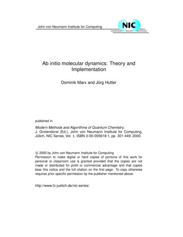
JDN 18171where the first four terms refer to intramolecular or local contributions to the total energy (bondstretching, angle bending, and dihedral and improper torsions), and the last two terms serve to describethe repulsive and Van der Waals interactions (in this case by means of a 12-6 Lennard-Jones potential)and the Coulombic interactions.2.2 Intramolecular termsAs shown in equation (2.1), bond stretching is very often represented with a simple harmonic functionthat controls the length of covalent bonds. Reasonable values for r0 can be obtained from X-raydiffraction experiments, while the spring constant may be estimated from infrared or Raman spectra.The harmonic potential is a poor approximation for bond displacements larger than 10% from theequilibrium value. Additionally the use of the harmonic function implies that the bond cannot bebroken, so no chemical processes can be studied. This is one of the main limitations of FF based MDsimulations compared to ab initio MD. Occasionally some other functional forms (in particular, theMorse potential) are employed to improve the accuracy. However as those forms are more expensivein terms of computing time and under most circumstances the harmonic approximation is reasonablygood, most of the existing potentials use the simpler harmonic function.Angle bending is also usually represented by a harmonic potential, although in some cases atrigonometric potential is preferred:1ka (cos cos 0 )2 .(2.2)2Some times other terms are added to optimize the fitting to vibrational spectra. The most commonaddition consists of using the Urey-Bradley potential [31]: 1UUB kUB (s s0 )2 ,(2.3)2anglesUbending where s is the distance between the two external atoms forming the angle.In any molecule containing more than four atoms in a row, we need to include also a dihedralor torsional term. While angle bending, and in particular bond stretching, are high frequency motionsthat often are not relevant for the study of the properties of interest and can be replaced by a rigidapproximation (see section 3.8), torsional motions are typically hundreds of times less stiff than bondstretching motions and they are necessary to ensure the correct degree of rigidity of the molecule and toreproduce the major conformational changes due to rotations about bonds. Therefore they play a crucialrole in determining the local structure of a macromolecule or the relative stability of different molecularconformations. As an example, the definition of a dihedral angle in the 1,2-dichloroethane molecule andthe corresponding torsional potential are shown in figures 1 and 2.Torsional energy is usually represented by a cosine function such as the one used in equation (2.1),where is the torsional angle, is the phase, n defines the number of minima or maxima between 0 and2 , and Vn determines the height of the potential barrier. The combination of two or more terms withdifferent n allows to construct a dihedral potential with minima having different depths. But alternativerepresentations for the dihedral potential can be found in the literature. For example the OPLS potentialuses the following expression [32]: k1k2k3k0 (1 cos ) (1 cos 2 ) (1 cos 3 ).Utors (2.4)222torsionsThe torsional parameters are usually derived from ab initio calculations and then refined usingexperimental data such as molecular geometries or vibrational spectra.Finally, an additional term is needed to ensure the planarity of some particular groups, such as sp2hybridized carbons in carbonyl groups or in aromatic rings. This is because the normal torsion terms
172Collection SFNFigure 1. Definition of the dihedral angle in 1,2-dichloroethane. The figure shows the gauche isomer.Figure 2. Torsional potential of 1,2-dichloroethane showing the gauche ( 60 and 300 ) and trans ( 180 )conformational isomers and the saddle points corresponding to the eclipsed conformations [33].described above are not sufficient to maintain planarity, so this extra component describes the positivecontribution to the energy of those out-of-plane motions. Typical expressions for the improper torsionterm are:Uimp kimp[1 cos(2 )],2impropersor
JDN 18Uimp kimp( 0 )2 ,2impropers173(2.5)where is the improper angle corresponding to the deviation from planarity.2.3 Intermolecular termsVan der Waals interactions between two atoms arise from the balance between repulsive and attractiveforces. Repulsion is due to the overlap of the electron clouds of both atoms, while the interactionsbetween induced dipoles result in an attractive component that varies as r 6 . The 12-6 Lennard-Jones(LJ) potential is very often used to represent these interactions, but it is not uncommon to find some“softer” terms to describe the repulsive part, in particular the exponential function, which is used in theBuckingham potential [34] and is preferred over the LJ function in studies of organic molecular crystals[35, 36]. Other functions used occasionally are the 9-6 LJ potential used in the COMPASS FF [37] oreven a buffered 14-7 LJ term, as employed in MMFF [38]. Van der Waals forces act between any pairof atoms belonging to different molecules, but they also intervene between atoms belonging to the samemolecule that are sufficiently separated, as described later. It is possible to define a set of parameters(e.g. ij and ij ) for each different pair of atoms, but for convenience most force fields give individualatomic parameters (i.e. i and i ), together with some rules to combine them. For example, for the LJpotential the corresponding depth of the well for the interaction between two atoms i and j is given bythe geometric mean, ij ( i j )1/2 , while the value at which the potential becomes zero can be given bythe geometric, ij ( i j )1/2 , or the arithmetic mean, ij 12 ( i j ), depending on the FF chosen.The final term in equation (2.1) serves to describe the electrostatic interactions. While the molecularelectronic density can be obtained with a high accuracy by means of high-level quantum-mechanicalcalculations, the problem of reducing such density to a manageable description to be used in a MDsimulation is not trivial. The usual choice is to assign a partial atomic charge to each nucleus and useCoulomb’s law to compute their contribution to the total energy. The partial charges can be derivedfrom a fit to experimental thermodynamic data, but this approach is only practical for small molecules[18]. There are also some fast methods to determine the charge distribution which are based on the atomelectronegativities [39–41]. However the most common way to obtain reliable partial charges consistsof performing an ab initio calculation and then deriving them from the quantum mechanical potential.Unfortunately they cannot be derived unambiguously because atomic charges are not experimentalobservables, so many different methods have been developed to determine them and they do not alwaysproduce the same distribution of partial charges [42, 43]. An important point to note is that in condensedphases there are polarization effects that cannot be fully described using fixed partial charges. Althoughpolarizable force fields exist (section 2.4), generally these non-pairwise additive effects are just takeninto account in an average way by using effective charges. As a consequence the resulting dipolemoment of a molecular model is usually larger than the experimental dipole moment correspondingto the isolated molecule. For example, most water models employ charge distributions giving 2.3–2.6 D instead of the experimental value for the vapour of 1.85 D [44]. Another point to note is thatelectrostatic interactions are long-ranged, so they require a particular treatment when truncating themin our computation of the forces. The techniques to deal with long-range interactions will be presentedin section 3.5. A final remark is that for computational efficiency and practical reasons, partial chargesare normally assigned only to the atomic sites. But nothing precludes placing them outside the atompositions. Again water gives us a good example, as we can find water models having only 3 sites (withpartial charges assigned to the O and H atoms), but also models with 4, 5 and even 6 sites [44].In most cases both the Van der Waals and electrostatic intramolecular interactions between atomsseparated by more than three bonds ( 1-4) are treated in the same way as if they were intermolecular,while interactions between 1-2 and 1-3 pairs are excluded. This is to avoid numerical problems, asthe potential can become strongly repulsive or attractive due to the small distances involved, and also
174Collection SFNbecause the interactions between those atoms are considered to be already correctly described by theintramolecular terms. The treatment of 1-4 interactions is less standard, but often they are partiallyexcluded by introducing a scaling factor. However the scaling can be different from one force field toanother. This has to be taken into account if parameters coming from different force fields are mixed.Furthermore it has to be considered that it is the particular combination of the dihedral potential withthe 1-4 Van der Waals and electrostatic interactions that determines the rotational barriers, so in generalit is not advised to modify them or to combine parameters coming from different sources.2.4 Special termsThe contributions to the energy described above appear in almost all force fields, but in certain cases wecan encounter some other additional terms.Thus it is possible to find cross terms describing the coupling between stretching, bending, andtorsion. They bring corrections to the intramolecular energy and allow to reproduce better the observedspectra of intramolecular vibrations. Examples of such cross-terms are:1kbb (r r0 )(r r0 ),2(2.6)1kba [(r r0 ) (r r0 )]( 0 ).2(2.7)Ubond bond Ubond bend Hydrogen bonding is usually reproduced by an adequate choice of van der Waals parameters and partialcharges, but some times an extra term is included to improve the accuracy of the H-bonding energy. ThisH-bonding potential may adopt different forms, but a general expression often used is [17]: AB 2cos AH D ,(2.8)UHB 1210rADrADwhere rAD is the distance between the donor and the acceptor, and AH D is the angle between the donor,the hydrogen, and the acceptor.Finally the most important addition to the standard potential given by eqn. (2.1) is the inclusionof polarization effects explicitly [45]. As explained above, local electric fields emerging in condensedphases will induce the appearance of dipoles. This is a non-pairwise additive interaction, so the useof effective charges to describe the average polarization is only a partial solution to this problem andfurthermore reduces the transferability of the FF. For example, the partial charges used to describe amolecule in the liquid state will not be adequate to describe the same molecule in the gas phase. Orthe same amino-acid should have different charge distributions in different proteins due to the differentelectrostatic environment. Furthermore the polarizability will affect the solvation energy of ions in anonpolar environment, the directionality and energetics of H-bonds, the interactions between cationsand aromatic molecules, etc. For this reason, most modern potentials include explicitly the polarization.In this case, for each atom or molecule the surrounding particles will induce a charge redistribution thatneeds to be modelled. There are three principal methods to do this [46, 47]:1. Fluctuating charges: The charges are allowed to fluctuate according to the environment, so thecharge flows between atoms until their instantaneous electronegativities are equal [48].2. Shell models (Drude particle): Electronic polarization is incorporated by representing the atomas the sum of a charged core and a charged shell connected by a harmonic spring whose forceconstant is inversely proportional to the atomic polarizability. The relative displacement of bothcharges depends on the electrostatic field created by the environment [49].3. Induced point dipoles: An induced point dipole i is associated to each polarizable atom:q i i (Ei Eindi ),(2.9)
JDN 18175qwhere i is the isotropic polarizability of the atom, Ei is the electrostatic field created on theatom i by the permanent charges, and Eindi is the field created by the induced dipoles of the rest ofthe atoms in the system.The polarization energy is:Upol 1 i Ei .2 i(2.10)As the induced dipoles depend both on the static charges and the remaining induced dipoles,they have to be determined self-consistently by solving the previous equations iteratively until thevalues for all the induced dipoles converge [50].Incorporating polarization effects into the potential describing the intermolecular interactions is animportant step forward. However a force field is a global entity, so the construction of new polarizableforce fields requires also a reoptimization of the Van der Waals and intramolecular parameters. Thisrepresents a huge task, so current polarizable force fields have not yet achieved a fully mature state [47].This could explain the unconvincing results obtained when comparing the ability of polarizable and nonpolarizable potentials to describe the structure of liquid water [51, 52]. Nevertheless recent comparisonson biological systems indicate that they are able to provide a better agreement with experiment than nonadditive force fields [47] and they provide a more physical representation of intermolecular interactions,increasing their transferability. Thus most of the new force fields currently being developed includepolarization effects in one way or another.2.5 Popular force fieldsThe first force fields appeared in the 1960’s, with the development of the molecular mechanics (MM)method and their primary goal was to predict molecular structures, vibrational spectra and enthalpies ofisolated molecules [17]. They were therefore mainly oriented to treat small organic molecules, but someof them have survived and continue to be developed and used today. The best example is given by theMM potentials developed by Allinger’s group [53]: MM2 [54], MM3 [55] and MM4 [56]. The first ofthese force fields was originally created to study hydrocarbons, but they were later extended to be ableto deal with many different types of organic or functionalized molecules (alcohols, ethers, sulphides,amides, etc.).Since then the scope of research has moved to deal with much more complex systems, leading to thedevelopment of more widely applicable force fields. Good examples are the Dreiding [57] and Universal(UFF) [58] force fields, that contain parameters for all the atoms in the periodic table. Other verypopular force fields are CHARMM [59], AMBER [60], GROMOS [61], OPLS [32], and COMPASS[37]. All of them are quite general, but the first three are often employed in simulations of biomolecules,while OPLS and COMPASS were originally developed to simulate condensed matter. It must also benoted that many of these force fields are continuously evolving and different versions are available(e.g. CHARMM19, CHARMM22, CHARMM27 [62]; GROMOS96, GROMOS45A3, GROMOS53A5,GROMOS53A6 [63]; AMBER91, AMBER94, AMBER96,AMBER99, AMBER02 [64]; etc.).The force fields using an energy expression similar to equation (2.1) are sometimes called firstgeneration or class I force fields. Second-generation or class II force field include the cross termsmentioned in section 2.4. COMPASS, UFF, MM2, MM3 and MM4 belong to this second class. Otherpopular class II force fields are CFF (consistent force field) [65] and MMFF (Merck molecular forcefield) [38].During the 1990s the first general polarizable force fields appeared. The PIPF (polarizableintermolecular potential function) [66], DRF90 [67] and AMOEBA [68] force fields are good examplesof such developments. In addition, some of the general force fields mentioned above have also developedpolarizable versions. Thus polarization has been introduced into CHARMM using either fluctuating
176Collection SFNcharges [69] or the shell model [70], and AMBER [71], OPLS [72] and GROMOS [73] have alsobeen extended to include polarization. A more comprehensive list of polarizable force fields is given inreference [47].In addition to those general force fields, there is a vast number of specific potentials developed todescribe just a particular system or a class of compounds. Water merits a particular mention in thisrespect, as due to its importance a large number of water models has been proposed since the first MCsimulation of Barker and Watts [74]. Many of those models are listed in reference [44], together witha critical review of their strengths and weaknesses. And recently Vega et al. performed an extensivecomparison of the most popular rigid non-polarizable water potentials (TIP3P, TIP4P, TIP5P, SPCand SPC/E), finding that a modified version of the second one, called TIP4P/2005, provides the bestdescription of 9 out of the 10 experimental properties investigated [75].It is even more difficult to compare the performance of the existing general force fields, as theresult will depend strongly on the system and properties simulated. Some comparisons can be foundin the literature, in particular concerning the accuracy of the CHARMM, AMBER and OPLS forcefields in the context of biomolecular simulations, but the results are not unambiguous. Thus Price andBrooks found that the three provided remarkably similar results concerning the structure and dynamicsof three different proteins [76]. On the other hand Yeh and Hummer found significant differencesin the configurations of two peptides studied with CHARMM and AMBER, as well as in the endto-end diffusion coefficient [77]. Aliev and Courtier-Murias also found a strong dependence of thestructure of small open chain peptides on the force field used [78]. A similar result was found insimulations of insulin using CHARMM, AMBER, OPLS, and GROMOS, as different structural trendsare favoured depending on the force field chosen [79]. One of the most detailed evaluation of existingpotentials has been performed by Paton and Goodman. They evaluated the interaction energies of 22molecular complexes of small and medium size and 143 nuclear acid bases and amino-acids usingseven different force fields (MM2, MM3, AMBER, OPLS , OPLSAA, MMFF94, and MMFF94s) andbenchmarked them against the energies obtained from high-level ab initio calculations. Their resultsshow that all the potentials tested, and specially OPLSAA and MMFF94s, describe quite accuratelyelectrostatic and van der Waals interactions, but that the magnitude of hydrogen bonding interactionsare severely underestimated [80]. The main conclusion is that each force field has its particular strengthsand weaknesses related to the data and procedure employed in its parametrization, so the final choicedepends on the particular problem being considered. However, as stated by Jorgensen and TiradoRives, “all leading force fields now provide reasonable results for a wide range of properties of isolatedmolecules, pure liquids, and aqueous solutions” [81].2.6 Parametrizing a force fieldThe ultimate goal of a force field is to describe in classical terms all the quantum mechanical facts,partitioning the total electronic energy into well separated atom-atom contributions, such as Coulombic,polarization, dispersion, and repulsive energies. Unfortunately, even disposing of very accurate QMcalculations, it is impossible to fully separate the intricate electronic effects (see reference [17]). Thisimplies that we are obliged to employ significant physical approximations in order to describe in atractable manner the intermolecular interactions, which limits their accuracy. Therefore they are calledempirical potentials or empirical force fields, and depending on the procedure followed to develop themand the set of input data used to optimize their parameters, we will obtain different force fields applicableto different systems or problems. This has led T. Halgren to say that “force field development is still asmuch a matter of art as of science” [82].From the above considerations, it should be clear that the development of a force field is not a trivialtask. A thorough account of the methodology needed to parametrize a general FF is given in the seriesof papers describing the Merck Molecular Force Field, MMFF94 [38, 83–86], and serves to exemplify
JDN 18177the complexity of this task. Here we will just mention the four basic steps needed to develop a new forcefield:1. Select the function to model the system energy: Are we going to employ cross-terms to describeintramolecular interactions? Shall we include polarization explicitly or is an additive potentialenough? What form are we going to use to represent van der Waals interactions (12-6 LJ, exponentialor other)?2. Choose the data set required to determine all the parameters needed in the previously selectedfunction: There is a large number of experimental data that can be employed, such as equilibriumbond lengths obtained from x-ray or neutron diffraction, force constants from vibrationalspectroscopy, heats of sublimation or vaporization, densities, etc. Nevertheless in many casesexperimental data are scarce or unreliable, so nowadays ab initio calculations constitute the mainsource of input data.3. Optimize the parameters: There is a large number of parameters, so very often they are refined instages. Additionally most of them are not decoupled, so a change in one value may affect someother parameter. Therefore the optimization becomes an iterative procedure. An alternative approachconsists in using a least-squares fitting to determine the whole set of parameters providing the bestagreement with the input information. Further details about both approaches are given in [18, 82] andreferences therein. Finally, a new and attractive approach is the force-matching method, consistingin directly fitting the potential energy surface derived from QM calculations [87, 88].4. Validate the final set of parameters by computing the properties of systems not employed in theparametrization procedure.This is an extremely hard and time-consuming job that is performed only by specialized groups, sothe end user normally only needs to select an appropriat
Force fields and molecular dynamics simulations M.A. González Institut Laue Langevin, 6 rue Jules Horowitz, 38042 Grenoble Cedex 9, France This paper reviews the basic concepts needed to understand Molecular Dynamics simulations and will hopefully serve as an introductory guide for the non-expert into this exciting topic. Abstract. The objective of this review is to serve as an introductory .