Transcription
An Adaptive CUSUM Chart for Drift Detection(Running title: CUSUM Chart for Drift Detection)Fan Yi and Peihua Qiu Department of Biostatistics, University of Florida, Gainesville, FL 32610, USA. Corresponding Author, E-mail: pqiu@ufl.eduAbstractIn practice, sequential processes often have gradual changes in their process distributionsover time. This is related to the drift detection problem in statistical process control. Inthe literature, there have been some existing discussions on this problem. But, most existingmethods are designed based on the assumption that the related drift is linear or have anotherspecific pattern. In reality, however, such specified patterns may not be valid. In this paper, wesuggest an adaptive CUSUM chart to handle the drift detection problem with a flexible driftpattern. The new method integrates the general framework to construct a CUSUM chart basedon the generalized likelihood ratio statistic and estimation of a shift size by the exponentiallyweighted least square regression procedure. Simulation studies show that the proposed methodis effective in various cases considered. The new method is also illustrated using an exampleabout the exchange rates between Indian Rupees and US Dollars.1Key Words: Adaptive CUSUM chart; Drift detection; Exponentially weighted least square;Likelihood ratio; Linear drift; Statistical process control.1IntroductionIn environmental science, scientists found that the gradual loss of water resource in certain regions(e.g., the Salton Sea region in California) was damaging the local environment and ecosystems forhuman beings, animals and plants (Shuford et al. 2002, 2004, Tiffany et al. 2007). In financial1The data used in the paper are available from the authors upon reasonable request.1
markets, exchange rates between two currencies would change gradually after the gradual adjustment of certain financial policies like interest rates (Zeileis et al. 2010). In such applications, thedistribution of the related response variable would have a drift after a certain time point, and it isimportant to detect such a drift as soon as possible so that some interventions can be implementedin a timely manner. This paper suggests a new and effective method for drift detection.In the SPC literature, most control charts are developed for detecting shifts in the distributionof a sequential process (Qiu 2014). There are also some existing discussions on detecting a meandrift for a sequential process (e.g., Gan 1992, Shu et al. 2008, Su et al. 2011, Zhou et al. 2010,Zou et al. 2009). For instance, Gan (1992) discussed the performance of the conventional CUSUMchart designed for detecting mean shifts when the process under monitoring actually had a linearmean drift. Shu et al. (2008) suggested a weighted CUSUM chart for detecting patterned meanshifts, including a linear drift. Su et al. (2011) discussed detection of a linear mean drift by usingan adaptive EWMA chart. Zhou et al. (2010) suggested a control chart for monitoring a processwith patterned mean or variance changes based on the generalized likelihood ratio statistic. Zouet al. (2009) compared several different control charts for detecting linear drifts, including theconventional CUSUM and EWMA charts, the generalized EWMA chart by Han and Tsung (2004),and two control charts based on the generalized likelihood ratio statistic under the linear drift andstep shift alternatives. While these research effort is important, the existing methods describedabove for drift detection still have much room for improvement because of the complexity of thedrift detection problem due to the facts that drifts can have many different patterns in practice,the existing methods were developed for detecting one or more specific patterns, and their specifieddrift patterns may not describe real drifts well in practice.In this paper, we propose a new method for drift detection. The new method uses the generalframework to construct a CUSUM chart based on the generalized likelihood ratio statistic, afterthe drift size at the current observation time is estimated by an exponentially weighted least squareregression procedure. Because the weights in the weighted least square regression procedure decay2
exponentially fast for past observations, the proposed CUSUM chart is robust to the actual driftpattern. Numerical studies show that this method performs favorably when compared with somerepresentative existing methods.The remainder of the paper is organized as follows. In Section 2, the proposed new methodis described in details. Its numerical performance is evaluated in Section 3 by some simulationexamples. Then, the method is demonstrated using an example about the exchange rates betweenIndian Rupees and US Dollars in Section 4. Several remarks conclude the paper in Section 5.2Proposed CUSUM ChartLet the process observation at time n be denoted as Xn , for n 1. When the process is in-control(IC) at n, assume that Xn N (µ0 , σ02 ), where µ0 and σ02 are the IC mean and variance. If theprocess is out of control (OC) at time n, then it is assumed that Xn N (µ0 δn σ0 , σ02 ), whereδn σ0 is the mean shift size. Let en (Xn µ0 )/σ0 be the standardized value of Xn , for n 1.Then, its IC and OC pdf functions are respectively1f0 (en ) exp( e2n /2),2π1f1 (en ) exp[ (en δn )2 /2],2πand the corresponding log likelihood ratio islog(f1 (en )/f0 (en )) δn (en δn /2).To detect such a mean shift, the conventional CUSUM charting statistic (cf., Qiu 2014, Section4.2.4) isCn max{0, Cn 1 δn (en δn /2)}, for n 1,where C0 0. From the above expression, it can be seen that the charting statistic Cn dependson δn which is often unknown in practice. To overcome this difficulty, we suggest estimating δn bythe following exponentially weighted least square regression procedure:nXmin(ei α βi)2 (1 λ)n i ,α,β Ri 13(1)
where λ [0, 1) is a weighting parameter. In (1), a line has been fitted to {ei , 0 i n} bya weighted least square regression procedure, and the weight (1 λ)n i at time i exponentiallydecays when i moves away from n. So, only observations whose observation times are close to nwould receive relatively large weights in this procedure.b Then, a reasonableLet the solutions to α and β in (1) be denoted respectively as αb and β.estimate of δn isbδbn αb βn.After δn is replaced by δbn in the expression of Cn , our suggested adaptive CUSUM chart fordetecting a mean drift ishibn max 0, Cbn 1 δbn (en δbn /2) , for n 1,C(2)b0 0. The chart gives a signal ifwhere Cbn h,C(3)where h 0 is a control limit. In the remaining part of the paper, this CUSUM chart is calledCUSUM-D chart, where “D” represents “drift”.From the construction of the CUSUM-D chart described above, it can be seen that the chartis constructed based on the log likelihood ratio statistic under the flexible OC framework that atime-varying shift of size δn σ0 occurs at time n. This OC framework contains all drift patterns,including the linear, quadratic and other types of drifts as special cases. To estimate δn by (1), theexponential weights (1 λ)n i used in (1) are meaningfully non-zero only at a few time points closeto n. Thus, the estimate δbn is actually local to n. For the reasons explained above, the CUSUM-Dchart should be robust to the mean drift pattern, which will be confirmed by a simulation examplein the next section.In the CUSUM-D chart (2)-(3), there are two parameters λ and h to determine in advance. Asin a conventional CUSUM or EWMA chart, the value of λ can be specified in advance, and then4
the control limit h can be determined easily by simulation to achieve a given ARL0 level. Selectionof λ will be studied numerically in the next section. To evaluate the performance of the CUSUM-Dchart, we can use the IC average run length, denoted as ARL0 , and the OC average run length,denoted as ARL1 , as discussed in Qiu (2014).3Simulation StudyThe simulation study is organized in two parts. First, selection of the parameter λ used in (1) isstudied carefully in a special case for detecting linear drifts in Subsection 3.1. Then, the IC andOC performance of the chart is studied in Subsection 3.2, in comparison with several representativeexisting methods.3.1Selection of λ used in (1).We study the impact of λ on the performance of the CUSUM-D chart when detecting linear driftsin this part. Results in such cases can provide some guidelines for selecting λ in other cases. First,it should be pointed out that selection of λ may depend on the shift time τ and the drift slopeγ. Consider cases when ARL0 200, the IC process distribution is N (0, 1), and the OC processdistribution is N (γ(n τ ), 1), for n τ . In the above setup, γ is allowed to change its valueamong {0.01 i, i 1, · · · , 30}, and τ is allowed to change among {20, 30, 40, 50, 60, 70}. For eachcombination of the γ and τ values, we search for the λ value so that the CUSUM-D chart has thesmallest ARL1 value, and the corresponding optimal λ value is denoted as λopt . In each case, theARL1 value is computed based on 10,000 replicated simulations. The results of the searched λoptvalues are shown in Figure 1. In the figure, the solid curve denotes λopt 2γ 3γ 2 , which is obtainedby the least square estimation when fitting a quadratic curve to the results shown in the last plotwhen τ 70. From the figure, we can have the following conclusions. First, when τ increases, theresults will stabilize, and can be described well by the function λopt 2γ 3γ 2 . This confirms that5
the CUSUM-D chart will enter the steady-state when the current observation time n increases, andthe relationship between λopt and γ can be described well by the quadratic function λopt 2γ 3γ 2 .Therefore, λ should be chosen larger when γ is larger, which is intuitively reasonable because theexponentially weighted least square regression procedure (1) should assign less weights to previousobservations whose observation times are far away from the current time n for detecting a steepermean drift. Second, when τ is small (e.g., τ 40), λ should be chosen according to the relationshipλopt 2γ 3γ 2 for detecting relatively steep mean drifts (e.g., γ 0.1), and 0 for detecting meandrifts that are quite flat, which is also intuitively reasonable.Figure 1: In each plot, small circles denote the optimal values of λ (i.e., λopt ), and the solid quadraticline denotes λopt 2γ 3γ 2 .3.2Comparison with several existing methodsIn this part, we evaluate the numerical performance of our proposed control chart CUSUM-D, incomparison with several representative existing charts. The first existing chart is the conventionalCUSUM chart, denoted as CUSUM (Page 1954). Readers are reminded that this conventionalCUSUM chart is designed for detecting step mean shifts, and optimal under the assumptions thatprocess observations at different time points are independent and identically normally distributed.The second existing chart is the GLR-L chart discussed in Zou et al. (2011), designed for detectinga linear mean drift using the classical likelihood ratio formulation for detecting a change-point. Thethird existing control chart considered is the ELM control chart proposed by Zhou et al. (2010).6
This chart integrates the EWMA charting statistic with the generalized likelihood ratio statisticfor monitoring a process with patterned mean or variance changes.IC Performance. We first investigate the IC performance of the four charts. In the conventional CUSUM chart, the allowance constant k is chosen to be the commonly used value of0.25. The weighting parameter is chosen to be 0.2 for the ELM chart and the CUSUM-D chart.The GLR-L chart is based on change-point detection, and does not have any parameter to choose.The assumed ARL0 value is chosen to be 200 for all four charts and their actual ARL0 values arecomputed by simulation as follows. First, we generate an IC dataset of size M from the N (0, 1)distribution. Then, the control limit is searched based on 5,000 bootstrap samples of the IC datasetuntil the assumed ARL0 value (i.e., 200) is reached. Then, the chart is applied to the sequentialobservations generated from the IC model, and an IC run length value can be computed. Thissequential monitoring process is repeated for 5,000 times, and the average of the 5,000 IC runlength values is calculated as the actual ARL0 value of the chart. We repeat the above processfor 100 times. The average of the 100 ARL0 values is used as the computed actual ARL0 valueof the chart. We consider cases when the IC sample size M 200, 500, 1, 000, 2, 000 and 5, 000.The computed actual ARL0 values of the four charts and their standard errors are presented inTable 1. From the table, it can be seen that i) the charts ELM and CUSUM-D have a reliable ICperformance in all cases considered, ii) the computed actual ARL0 value of the chart CUSUM isbeyond 5% of the nominal ARL0 value of 200 when M 200 and within 5% of the nominal ARL0value when M 500, and iii) the chart GLR-L has an unreliable IC performance when M 200and becomes reliable when M 500. This example confirms that all four charts have a reliable ICperformance when M 500, and the charts ELM and CUSUM-D have a reliable IC performanceeven when M 200.OC Performance. To evaluate the OC performance of the four charts described above,we consider cases when τ 50, and Xn N (γ1 (n τ ), 1) (i.e., linear mean drift) or Xn N (γ2 (n τ )2 , 1) (i.e., quadratic mean drift), for n τ , after the process becomes OC. Other setups7
Table 1: Actual ARL0 values and their standard errors (in parentheses) of the four charts CUSUM,GLR-L, ELM and CUSUM-D in cases when the IC sample size M 200, 500, 1, 000, 2, 000, or5, 000.M200CUSUMGLR-LELMCUSUM-D216.36(11.73) 128.27(6.55) 203.22(12.21) 205.87(11.51)500205.40(1.03) 89) 74) 34) 199.91(2.59)202.58(2.38)202.12(2.42)are the same as those in the example of Figure 1 above. For each chart, its nominal ARL0 valueis fixed at 200, and its control limit is chosen based on 10,000 IC process observations generatedfrom the N (0, 1) distribution. To make the comparison among different charts fair, for detectinga given mean drift, the procedure parameters of each chart are chosen such that its ARL1 valuereaches the minimum. Namely, the optimal performance of the charts is compared here, which isrecommended in the literature (cf., Qiu et al. 2020). In each case, the optimal ARL1 value of achart is computed based on 10,000 replicated simulations. The computed ARL1 values of the fourcharts for detecting some linear mean drifts are presented in Table 2, and the corresponding resultsfor detecting some quadratic mean drifts are presented in Table 3. From the tables, we can havethe following conclusions. First, the proposed new chart CUSUM-D performs the best in all casesconsidered for detecting linear mean drifts, compared to the three competing methods. It is betterthan the conventional CUSUM chart because the latter is optimal for detecting step shifts only,and the former is designed for detecting mean drifts that is considered in this example. Second, itcan be seen that the chart CUSUM-D is also the best among all four charts for detecting quadraticmean drifts. Thus, its performance is indeed quite robust to the mean drift patterns. Third, bychecking the results of the other three charts, it can be seen that the charts GLR-L and ELM do8
not perform well, especially when the mean drifts are relatively small. This conclusion is actuallyconsistent with the results in Zhou et al. (2010) and Zou et al. (2011) which confirmed that thecharts GLR-L and ELM performed well only when the mean drifts were large. This example showsthat CUSUM-D is indeed effective for detecting mean drifts and quite robust to the mean driftpatterns.Table 2: Optimal ARL1 values with standard errors (in parenthesis) of the four control charts fordetecting some linear mean drifts when τ 50 and ARL0 200. Number in bold in each rowdenotes the smallest ARL1 value in that row.γ1CUSUMGLR-LELMCUSUM-D0.001 98.93(0.72) 138.39(1.41) 104.79(0.99) 81.65(3.63)0.005 52.30(0.38)70.05(0.66)53.61(0.48) 43.57(2.34)0.0137.65(0.31)48.54(0.48)38.11(0.35) 32.74(2.00)0.0516.11(0.22)18.92(0.27)16.22(0.20) 15.38(1.48)0.110.87(0.21)12.39(0.23)10.92(0.18) 10.67(0.36)Table 3: Optimal ARL1 values with standard errors (in parenthesis) of the four control charts fordetecting some quadratic mean drifts when τ 50 and ARL0 200. Number in bold in each rowdenotes the smallest ARL1 value in that row.γ2CUSUMGLR-LELMCUSUM-D0.0001 54.26(0.40) 63.90(0.58) 54.69(0.46) 45.73(2.39)0.0005 32.82(0.30) 37.38(0.38) 32.89(0.30) 29.48(1.89)0.00126.06(0.26) 29.28(0.33) 26.12(0.26) 24.03(1.73)0.00514.88(0.23) 16.10(0.25) 14.90(0.20) 14.44(1.45)0.0111.61(0.21) 12.42(0.23) 11.65(0.19) 11.44(0.35)9
4An ApplicationIn this section, we apply the proposed control chart CUSUM-D and the three alternative chartsCUSUM, GLR-L and ELM to a real-data example about the daily exchange rates between IndianRupee and US Dollar between Nov 01, 2010 and December 30, 2011. There are a total of 292exchange rates during this time period, and they are shown in the left panel of Figure 2. Fromthe plot, it can be seen that the first 200 observations are quite stable, compared with the last 92observations, where the two groups of observations are separated by the vertical dashed line. So,the first 200 observations are used as IC data, and the remaining ones are used for online processmonitoring.From Section 2, the current version of the proposed CUSUM-D chart is constructed basedon the assumptions that the process distribution is normal and the process observations at different time points are independent of each other. To check these assumptions, the R functionsshapiro.test() and Box.test() are used for testing for the normality and autocorrelation of theIC data, respectively. The p-values of these two tests are 0.039 and 0.001. Thus, the distributionof the IC data is significantly different from normal, and there is a significant serial data correlationin the IC data. To decorrelate the data, the serial data correlation structure is first estimated fromthe IC data, and then the recursive data decorrelation procedure discussed in Qiu et al. (2020) isused to decorrelate all observed data. To transform the decorrelated data so that the distributionof the transformed data becomes normal, we consider using the Johnson’s transformation families(Johnson 1949, Slifker and Shapiro 1980) via the R function jtrans(). After data decorrelation andnormalization, the R functions shapiro.test() and Box.test() are applied to the IC data again,and the p-values of these two tests are 0.936 and 0.887, respectively. Thus, the serial data correlation has been mostly deleted by the data decorrelation procedure, and the normality assumptionis valid now after using the Johnson’s transformation. The decorrelated and normalized data areshown in the right panel of Figure 2.10
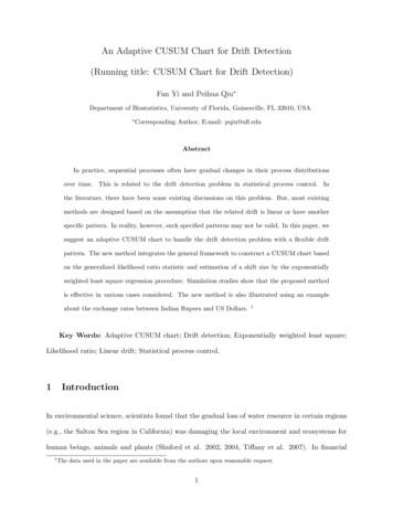
Figure 2: Left panel shows the original observations of the exchange rates between Indian Rupeeand US Dollar during Nov 01, 2010 and December 30, 2011. Right panel shows the decorrelatedand normalized data. The vertical dashed line in each plot separates the IC data and the data foronline process monitoring, and the horizontal dashed line denotes the IC mean.Next, we apply the proposed CUSUM-D chart to this data, together with the alternative chartsCUSUM, GLR-L and ELM. In CUSUM-D, we set λ 0 based on the simulation results shown inFigure 1 and the expectation that a mean drift can occur anytime soon after the online processmonitoring starts. In the conventional CUSUM chart, the allowance constant k is chosen to be thecommonly used value of 0.25. For the ELM control chart, the weighting parameter λe is chosento be 0.2, as suggested in Zhou et al. (2010). The related charts are shown in Figure 3. TheCUSUM, GLR-L, ELM and CUSUM-D charts give their first signals on 09/07/2011, 09/09/2011,09/08/2011 and 09/06/2011, respectively. So, the CUSUM-D chart gives the earliest signal in thisexample. The detected upward drift should be related to the S&P downgrade of the credit rating ofthe United States from AAA to AA on August 5, 2011. This example shows that the CUSUM-Dchart is quite effective in detecting such mean drifts.11
Figure 3: The four control charts when they are used for monitoring the decorrelated and normalizedexchange rates between the Indian Rupee and US Dollar during 08/18/2011 and 10/28/2011.5Concluding RemarksWe have described a new control chart for detecting process mean drifts. The new method isconstructed based on the generalized likelihood ratio statistic and the exponentially weighted leastsquare estimation of a mean shift size. Numerical studies have confirmed that it is effective indetecting mean drifts in different cases considered. While our proposed chart CUSUM-D has beenshown to perform the best, compared to its three peers, in the numerical studies presented inSection 3, we would like to remind the readers that this chart is designed for detecting mean driftswith unknown drift patterns. For detecting mean shifts, for example, the conventional CUSUM12
chart or its modified versions should be considered. The current version of the proposed methodis designed for cases when the process distribution is normal and process observations at differenttime points are independent of each other. In cases when the normality assumption is invalid,a nonparametric version of the proposed method might be possible by using data categorizationor other approaches for constructing nonparametric control charts (e.g., Qiu and Li 2011). Incases when the observed data are serially correlated, a time series model or a data decorrelationprocedure by moment estimation of the serial data correlation might be used to remove the serialdata correlation (e.g., Apley and Tsung 2002, Qiu et al. 2020) first, and then the proposed methodcan be used afterwards. Also, the steady-state relationship between λopt and γ for detecting lineardrifts is obtained in Section 3.1 by numerical studies only. Theoretical justification of that resultis needed. All these problems will be studied carefully in our future research.Acknowledgments: The authors thank the editor and a referee for some constructive comments and suggestions which improved the quality of the paper greatly. This research is supportedin part by an NSF grant with the grant number DMS-1914639.ReferencesApley D.W., and Tsung, F. (2002), “The autoregressive T 2 chart for monitoring univariate autocorrelated processes,” Journal of Quality Technology, 34, 80–96.Gan, F.F. (1992), “CUSUM control charts under linear drift,” The Statistician, 41, 71–84.Han, D., and Tsung, F. (2004), “A generalized EWMA control chart and its comparison with theoptimal EWMA, CUSUM and GLR schemes,” The Annals of Statistics, 32, 316–339.Johnson, N.L. (1949), “Systems of frequency curves generated by methods of translation,” Biometrika,36, 149–176.Page, E.S. (1954), “Continuous inspection schemes,” Biometrika, 41, 100–115.13
Qiu, P. (2014), Introduction to Statistical Process Control, Boca Raton, FL: Chapman Hall/CRC.Qiu, P., and Li, Z. (2011), “On nonparametric statistical process control of univatiate processes,”Technometrics, 53, 390–405.Qiu, P., Li, W., and Li, J. (2020), “A new process control chart for monitoring short-range seriallycorrelated data,” Technometrics, 62, 71–83.Shu, L., Jiang, W., and Tsui, K.L. (2008), “A weighted CUSUM chart for detecting patternedmean shifts,” Journal of Quality Technology, 40, 194–213.Shuford, W.D., Warnock, N., Molina, K.C., and Sturm, K. (2002), “The Salton Sea as criticalhabitat to migratory and resident waterbirds,” Hydrobiologia, 473, 255–274.Slifker J.F., and Shapiro, S.S. (1980), “The johnson system: selection and parameter estimation,”Technometrics, 22, 239–246.Su, Y., Shu, L., and Tsui, K.L. (2011), “Adaptive EWMA procedures procedures for monitoringprocesses subject to linear drifts,” Computational Statistics and Data Analysis, 55, 2819–2829.Tiffany, M.A., Ustin, S.L., and Hurlbert, S.H. (2007), “Sulfide irruptions and gypsum blooms inthe Salton Sea as detected by satellite imagery, 1979-2006,” Lake and Reservoir Management,23, 637–652.Zeileis, A., Shah, A., and Patnaik, I. (2010), “Testing, monitoring, and dating structural changesin exchange rate regimes,” Computational Statistics & Data Analysis, 54, 1696–1706.Zhou, Q., Luo, Y.Z., and Wang, Z. (2010), “A control chart based on likelihood ratio test fordetecting patterned mean and variance shifts,” Computational Statistics and Data Analysis,54, 1634–1645.Zou, C., Liu, Y., and Wang, Z. (2009), “Comparisons of control schemes for monitoring the meanof processes subject to drifts,” Metrika, 70, 141–163.14
CUSUM chart is designed for detecting step mean shifts, and optimal under the assumptions that process observations at di erent time points are independent and identically normally distributed. The second existing chart is the GLR-L chart discussed in Zou et al. (2011), designed for detecting .