Transcription
Contemporary MathematicsEliminating Human Insight: An Algorithmic Proof ofStembridge’s TSPP TheoremChristoph KoutschanAbstract. We present a new proof of Stembridge’s theorem about the enumeration of totally symmetric plane partitions using the methodology suggested in the recent Koutschan-Kauers-Zeilberger semi-rigorous proof of theAndrews-Robbins q-TSPP conjecture. Our proof makes heavy use of computeralgebra and is completely automatic. We describe new methods that make thecomputations feasible in the first place. The tantalizing aspect of this work isthat the same methods can be applied to prove the q-TSPP conjecture (thatis a q-analogue of Stembridge’s theorem and open for more than 25 years); theonly hurdle here is still the computational complexity.1. IntroductionThe theorem (see Theorem 2.3 below) that we want to address in this paperis about the enumeration of totally symmetric plane partitions (which we will abbreviate as TSPP, the definition is given in Section 2); it was first proven by JohnStembridge [8]. We will reprove the statement using only computer algebra; thismeans that basically no human ingenuity (from the mathematical point of view) isneeded any more—once the algorithmic method has been invented (see Section 3).But it is not as simple (otherwise this paper would be needless): The computationsthat have to be performed are very much involved and we were not able to do themwith the known methods. One option would be to wait for 20 years hoping thatMoore’s law equips us with computers that are thousands of times faster than theones of nowadays and that can do the job easily. But we prefer a second option,namely to think about how to make the problem feasible for today’s computers.The main focus therefore is on presenting new methods and algorithmic aspectsthat reduce the computational effort drastically (Section 4). Our computations(for the details read Section 5) were performed in Mathematica using our newlydeveloped package HolonomicFunctions [6]; this software is available on the RISCcombinatorics software at/software/HolonomicFunctions/2000 Mathematics Subject Classification. Primary 05A17, 68R05.supported by grant P20162 of the Austrian FWF.c 0000 (copyright holder)1
2CHRISTOPH KOUTSCHANSomehow, our results are a byproduct of a joint work with Doron Zeilbergerand Manuel Kauers [5] where the long term goal is to apply the algorithmic proofmethod to a q-analogue of Theorem 2.3 (see also Section 6). The ordinary (q 1)case serves as a proof-of-concept and to get a feeling for the complexity of theunderlying computations; hence it delivers valuable information that go beyondthe main topic of this paper.Before we start we have to agree on some notation: We use the symbol Sn todenote the shift operator, this means Sn f (n) f (n 1) (in words “Sn applied tof (n)”). We use the operator notation for expressing and manipulating recurrencerelations. For example, the Fibonacci recurrence Fn 2 Fn 1 Fn translatesto the operator Sn2 Sn 1. When we do arithmetic with operators we have totake into account the commutation rule Sn n (n 1)Sn , hence such operatorscan be viewed as elements in a noncommutative polynomial ring in the indeterminates n1 , . . . , nd and Sn , . . . , Snd . Usually we will work with a structure called Orealgebra, this means we consider an operator as a polynomial in Sn1 , . . . , Snd withcoefficients being rational functions in n1 , . . . , nd . Note that the noncommutativitynow appears between the indeterminates of the polynomial ring and the coefficients.In this context when speaking about the support of an operator we refer to the setof power products (monomials) in the Sni whose coefficient is nonzero. For a givensequence we can consider the set of all recurrences that this sequence fulfills; theyform a left ideal in the corresponding operator algebra. We call it annihilating idealor in short annihilator of the sequence. A sequence is called -finite if there existsan annihilating ideal with the property that only finitely many monomials can notbe reduced by it, in other words if the set of monomials that lie under the staircaseof a Gröbner basis of the ideal is finite. Together with the appropriate set of initialvalues we refer to it as a -finite description of the sequence.2. Totally Symmetric Plane PartitionsIn this section we want to give a short motivation of the combinatorial background of our problem.Definition 2.1. A plane partition π of some integer n is a two-dimensionalarrayπ (πij ), πij N for integers i, j 1Pwith finite sum n i,j 1 πij which is weakly decreasing in rows and columns, ormore preciselyπi 1,j πijand πi,j 1 πijfor all i, j 1.Note that this definition implies that only finitely many entries πij can benonzero. To each plane partition we can draw its 3D Ferrers diagram by stacking πijunit cubes on top of the location (i, j). Each unit cube can be addressed by itslocation (i, j, k) in 3D coordinates. A 3D Ferrers diagram is a justified structure inthe sense that if the position (i, j, k) is occupied then so are all positions (i0 , j 0 , k 0 )with i0 i, j 0 j, and k 0 k. Figure 1 shows an example of a plane partitiontogether with its 3D Ferrers diagram. We are now going to define TSPPs, theobjects of interest.Definition 2.2. A plane partition is totally symmetric iff whenever the position (i, j, k) in its 3D Ferrers diagram is occupied (in other words πij k), it
AN ALGORITHMIC PROOF OF STEMBRIDGE’S TSPP THEOREM54132131Figure 1. A plane partition of n 17follows that all its permutations {(i, k, j), (j, i, k), (j, k, i), (k, i, j), (k, j, i)} are alsooccupied.Now Stembridge’s theorem [8] can be easily stated:Theorem 2.3. The number of totally symmetric plane partitions whose 3D Ferrers diagram is contained in the cube [0, n]3 is given by the nice product-formulaYi j k 1(2.1).i j k 21 i j k nExample 2.4. We are considering the case n 2:there should beY2 3 4i j k 1 · ·i j k 21 2 31 i j k 2Formula (2.1) tells us that·5 54TSPPs inside the cube [0, 2]3 which is confirmed by the enumeration given in Figure 2.As others that proved the TSPP formula before us we will make use of aresult by Soichi Okada [7] that reduces the proof of Theorem 2.3 to a determinantevaluation:Theorem 2.5. The enumeration formula (2.1) for TSPPs is correct if and onlyif the determinant evaluation 2Yi j k 1(2.2)det (a(i, j))1 i,j n i j k 21 i j k nholds, where the entries in the matrix are given by i j 2i j 1(2.3)a(i, j) 2δ(i, j) δ(i, j 1).i 1iIn the above, δ(i, j) denotes the Kronecker delta.Ten years after Stembridge’s proof, George Andrews, Peter Paule, and CarstenSchneider [1] came up with a computer-assisted proof. They transformed the problem into the task to verify a couple of hypergeometric multiple-sum identities (whichthey could do by the computer). This problem transformation however required
4CHRISTOPH KOUTSCHANFigure 2. All TSPPs that fit into the cube [0, 2]2human insight. We claim to have the first “human-free” computer proof of Stembridge’s theorem that is completely algorithmic and does not require any humaninsight into the problem. Moreover our method generalizes immediately to theq-case which is not so obvious to achieve in the approach presented in [1].3. Proof method for determinant evaluationsDoron Zeilberger [13] proposes a method for completely automatic and rigorousproofs of determinant evaluations that fit into a certain class. For the sake ofself-containedness this section gives a short summary how the method works. Itaddresses the problem: For all n 0 prove thatdet(a(i, j))1 i,j n Nice(n),for some explicitly given expressions a(i, j) and Nice(n). What you have to do is thefollowing: Pull out of the hat another discrete function B(n, j) (this looks a littlebit like magic for now—we will make this step more explicit in the next section)and check the identitiesnX(3.1)B(n, j)a(i, j) 0 for 1 i n, i, n N,j 1(3.2)B(n, n) 1for all n 1,n N.Then by uniqueness, it follows that B(n, j) equals the cofactor of the (n, j) entryof the n n determinant (i.e. the minor with the last row and the jth columnremoved, this means we expand the determinant with respect to the last row usingLaplace’s formula), divided by the (n 1) (n 1) determinant. In other words wenormalized in a way such that the last entry B(n, n) is 1. Or, to make the argumenteven more explicit: What happens if we replace the last row of the matrix by anyof the other rows? Clearly then the determinant will be zero; and nothing else isexpressed in equation (3.1).
AN ALGORITHMIC PROOF OF STEMBRIDGE’S TSPP THEOREMFinally one has to verify the identitynXNice(n)(3.3)B(n, j)a(n, j) Nice(n 1)j 1for all n 1,5n N.If the suggested function B(n, j) does satisfy all these identities then the determinant identity follows immediately as a consequence.4. The algorithmsWe now explain how the existing algorithms (in short) as well as our approach(in more detail) find a recurrence for some definite sum. In order to keep thedescriptions simple and concrete we consider a sum of the formnXf (n, j)j 1as it appears in (3.3) (everything generalizes to instances with more parameters inthe summand as it is the case in (3.1)). We give some indications why the existingalgorithms fail to work in practice; all these statements refer to (3.3) but apply ina similar fashion to (3.1) as well.4.1. Some unsuccessful tries. There are several methods in the literaturehow to algorithmically prove identities like (3.1) and (3.3). The first one traces backto Doron Zeilberger’s seminal paper [12] and he later named it the slow algorithm.The idea is to find a recurrence operator in the annihilating ideal of the summandthat does not contain the summation variable in its coefficients; such a relation canalways be rewritten in the formP (n, Sn ) (Sj 1)Q(n, Sj , Sn )and we call P the principal part and Q the delta part. Such a telescoping relationencodes that P is a recurrence for the sum (depending on the summand and thedelta part we might have to add an inhomogeneous part to this recurrence). Theelimination can be performed by a Gröbner basis computation with appropriateterm order. In order to get a handle on the variable j we have to consider therecurrences as polynomials in j, Sj , and Sn with coefficients in Q(n) (for efficiencyreasons this is preferable compared to viewing the recurrences as polynomials in all4 indeterminates with coefficients in Q). We tried this approach but it seems to behopeless: The variable j that we would like to eliminate occurs in the annihilatingrelations for the summand B(n, j)a0 (n, j) with degrees between 24 and 30. Whenwe follow the intermediate results of the Gröbner basis computation we observethat none of the elements that were added to the basis because some S-polynomialdid not reduce to zero has a degree in j lower than 23 (we aborted the computationafter more than 48 hours). Additionally the coefficients grow rapidly and it seemsvery likely that we run out of memory before coming to an end.The second option that we can try is often referred to as Takayama’s algorithm [9]. In fact, we would like to apply a variant of Takayama’s original algorithmthat was proposed by Chyzak and Salvy [3]. Concerning speed this algorithm ismuch superior to the elimination algorithm described above: It computes only theprincipal part P of some telescoping operator(4.1)P (n, Sn ) (Sj 1)Q(j, n, Sj , Sn ).
6CHRISTOPH KOUTSCHANWhen we sum over natural boundaries we need not to know about the delta part Q.This is for example the case when the summand has only finite support (which is thecase in our application). Also this algorithm boils down to an elimination problemwhich, as before, seems to be unsolvable with today’s computers: We now can lowerthe degree of j to 18, but the intermediate results consume already about 12GB ofmemory (after 48 hours).The third option is Chyzak’s algorithm [2] for -finite functions: It finds arelation of the form (4.1) by making an ansatz for P and Q; the input recurrencesare interpreted as polynomials in Sj and Sn with coefficients being rational functionsin j and n. It uses the fact that the support of Q can be restricted to the monomialsunder the stairs of the input annihilator and it loops over the order of P . Becauseof the multiplication of Q by Sj 1 we end up in solving a coupled linear system ofdifference equations for the unknown coefficients of Q. Due to the size of the input,we did not succeed in uncoupling this system, and even if we can do this step, itremains to solve a presumably huge (concerning the size of the coefficients as wellas the order) scalar difference equation.4.2. A successful approach. The basic idea of what we propose is verysimple: We also start with an ansatz in order to find a telescoping operator. Butin contrast to Chyzak’s algorithm we avoid the expensive uncoupling and solvingof difference equations. The difference is that we start with a polynomial ansatzin j up to some degree:(4.2)IXci (n)Sni(Sj 1) ·K XL XMXdk,l,m (n)j k Sjl Snm .k 0 l 0 m 0i 0 {z P (n,Sn )} {z Q(j,n,Sj ,Sn )}The unknown functions ci and dk,l,m to solve for are rational functions in n andthey can be computed using pure linear algebra. Recall that in Chyzak’s algorithmwe have to solve for rational functions in n and j which causes the system tobe coupled. The prize that we pay is that the shape of the ansatz is not at allclear from a priori: The order of the principal part, the degree bound for thevariable j and the support of the delta part need to be fixed, whereas in Chyzak’salgorithm we have to loop only over the order of the principal part. Our approachis similar to the generalization of Sister Celine Fasenmyer’s technique that is usedin Wegschaider’s MultiSum package [11] (which can deal with multiple sums butonly with hypergeometric summands). We proceed by reducing the ansatz witha Gröbner basis of the given annihilating left ideal for the summand, obtaininga normal form representation of the ansatz. Since we wish this relation to be inthe ideal, the normal form has to be identically zero. Equating the coefficients ofthe normal form to zero and performing coefficient comparison with respect to jdelivers a linear system for the unknowns that has to be solved over Q(n).Trying out for which choice of I, K, L, M the ansatz delivers a solution can bea time-consuming tedious task. Additionally, once a solution is found it still canhappen that it does not fit to our needs: It can well happen that all ci are zero inwhich case the result is useless. Hence the question is: Can we simplify the searchfor a good ansatz, for example, by using homomorphic images? Clearly we canreduce the size of the coefficients by computing modulo a prime number (we mayassume that the input operators have coefficients in Z[j, n], otherwise we can clear
AN ALGORITHMIC PROOF OF STEMBRIDGE’S TSPP THEOREM7denominators). But in practice this does not reduce the computational complexitytoo much—still we have bivariate polynomials that can grow dramatically duringthe reduction process. For sure we can not get rid of the variable j since it isneeded later for the coefficient comparison. It is also true that we can not just plugin some concrete integer for n: We would lose the feature of noncommutativitythat n shares with Sn (recall that Sn n (n 1)Sn , but Sn 7 7Sn for example).And the noncommutativity plays a crucial role during the reduction process, in thesense that omitting it we get a wrong result. Let’s have a closer look what happensand recall how the normal form computation works:Algorithm: Normal form computationInput: an operator p and a Gröbner basis G {g1 , . . . , gm }Output: normal form of p modulo the left ideal hGiwhile exists 1 i m such that lm(gi ) lm(p)g : (lm(p)/lm(gi )) · gip : p (lc(p)/lc(g)) · gend whilereturn pwhere lm and lc refer to the leading monomial and the leading coefficient of anoperator respectively.Note that we do the multiplication of the polynomial that we want to reducewith in two steps: First multiply by the appropriate power product of shift operators(line 2), and second adjust the leading coefficient (line 3). The reason is becausethe first step usually will change the leading coefficient. Note also that p is nevermultiplied by anything. This gives rise to a modular version of the normal formcomputation that does respect the noncommutativity.Algorithm: Modular normal form computationInput: an operator p and a Gröbner basis G {g1 , . . . , gm }Output: modular normal form of p modulo the left ideal hGiwhile exists 1 i m such that lm(gi ) lm(p)g : h((lm(p)/lm(gi )) · gi )p : p (lc(p)/lc(g)) · gend whilereturn pwhere h is an insertion homomorphism, in our example h : Q(j, n) Q(j),h(f (j, n)) 7 f (j, n0 ) for some n0 N. Thus most of the computations are donemodulo the polynomial n n0 and the coefficient growth is moderate compared tobefore (univariate vs. bivariate).Before starting the non-modular computation we make the ansatz as small aspossible by leaving away all unknowns that are 0 in the modular solution. Withvery high probability they will be 0 in the final solution too—in the opposite casewe will realize this unlikely event since then the system will turn out to be unsolvable. In [11] a method called Verbaeten’s completion is used in order to recognizesuperfluous terms in the ansatz a priori. We were thinking about a generalizationof that, but since the modular computation is negligibly short compared to the rest,we don’t expect to gain much and do not investigate this idea further.
8CHRISTOPH KOUTSCHANOther optimizations concern the way how the reduction is performed. With abig ansatz that involves hundreds of unknowns (as it will be the case in our work)it is nearly impossible to do it in the naive way. The only possibility to achieve theresult at reasonable cost is to consider each monomial in the support of the ansatzseparately. After having computed the normal forms of all these monomials we cancombine them in order to obtain the normal form of the ansatz. Last but not leastit pays off to make use of the previously computed normal forms. This means thatwe sort the monomials that we would like to reduce according to the term orderin which the Gröbner basis is given. Then for each monomial we have to performone reduction step and then plug in the normal forms that we have already (sinceall monomials that occur in the support after the reduction step are smaller withrespect to the chosen term order).5. The computer proofWe are now going to give the details of our computer proof of Theorem 2.3following the lines described in the previous section.5.1. Get an annihilating ideal. The first thing we have to do according toZeilberger’s algorithmic proof technique is to resolve the magic step that we haveleft as a black box so far, namely “to pull out of the hat” the sequence B(n, j)for which we have to verify the identities (3.1) – (3.3). Note that we are able,using the definition of what B(n, j) is supposed to be (namely a certain minorin a determinant expansion), to compute the values of B(n, j) for small concreteintegers n and j. This data allows us (by plugging it into an appropriate ansatzand solving the resulting linear system of equations) to find recurrence relationsfor B(n, j) that will hold for all values of n and j with a very high probability. Wecall this method guessing; it has been executed by Manuel Kauers who used hishighly optimized software Guess.m [4]. More details about this part of the proofcan be found in [5]. The result of the guessing were 65 recurrences, their total sizebeing about 5MB.Many of these recurrences are redundant and it is desirable to have a uniquedescription of the object in question that additionally is as small as possible (ina certain metric). To this end we compute a Gröbner basis of the left ideal thatis generated by the 65 recurrences. The computation was executed by the author’s noncommutative Gröbner basis implementation which is part of the packageHolonomicFunctions. The Gröbner basis consists of 5 polynomials (their totalsize being about 1.6MB). Their leading monomials Sj4 , Sj3 Sn , Sj2 Sn2 , Sj Sn3 , Sn4 form astaircase of regular shape. This means that we should take 10 initial values intoaccount (they correspond to the monomials under the staircase).In addition, we have now verified that all the 65 recurrences are consistent.Hence they are all describing the same object. But since we want to have a rigorousproof we have to admit at this point that what we have found so far (that is a finite description of some bivariate sequence—let’s call it B 0 (n, j)) does not proveanything yet. We have to show that this B 0 (n, j) is identical to the sequence B(n, j)defined by (3.1) and (3.2). Finally we have to show that identity (3.3) indeed holds.5.2. Avoid singularities. Before we start to prove the relevant identitiesthere is one subtle point that, aiming at a fully rigorous proof, we should not omit:the question of singularities in the -finite description of B 0 (n, j). Recall that in
AN ALGORITHMIC PROOF OF STEMBRIDGE’S TSPP THEOREM9njFigure 3. The points for which the initial values of the sequenceB(n, j) have to be given because the recurrences do not apply.the univariate case when we deal with a P-finite recurrence, we have to regard thezeros of the leading coefficient and in case that they introduce singularities in therange where we would like to apply the recurrence, we have to separately specifythe values of the sequence at these points. Similarly in the bivariate case: Wehave to check whether there are points in N2 where none of the recurrences canbe applied because the leading term vanishes. For all points that lie in the area(4, 4) N2 we may apply any of the recurrences, hence we have to look for commonnonnegative integer solutions of all their leading coefficients. A (commutative)Gröbner basis computation reveals that everything goes well: From the first elementof the Gröbner basis(n 3)2 (n 2)(n 1)2 (2n 3)2 (2n 1)(j n 1)(j n)we can read off the solutions (0, 0), (1, 0), and (0, 1) (which are also solutions ofthe remaining polynomials but since they are lying under the stairs they are ofno interest). Further we have to address the cases n 1, 2, 3. Plugging theseinto the remaining polynomials we obtain further common solutions: (1, 1), (2, 1),(2, 2), (3, 2), and (3, 3). But all of them are outside of (4, 4) N2 so we need notto care. It remains to look at the lines j 0, 1, 2, 3 and the lines n 0, 1, 2, 3(we omit the details here; the corresponding univariate problems are easy to solve).Summarizing, the points for which initial values have to be given (either becausethey are under the stairs or because of singularities) are{(j, n) 0 j 6 0 n 1} {(j, 2) 0 j 4} {(j, 3) 0 j 3} {(j, 4) 0 j 2} {(1, 5)}.They are depicted in Figure 3. Note that only now we have a complete descriptionof the sequence B(n, j) and that again Gröbner bases played a crucial role to achievethis.5.3. The second identity. The simplest of the three identities to prove is(3.2). From the -finite description of B 0 (n, j) we can compute a recurrence for thediagonal B 0 (n, n) by the closure property “substitution”. HolonomicFunctionsdelivers a recurrence of order 7 in a couple of minutes. Reducing this recurrencewith the ideal generated by Sn 1 (which annihilates 1) gives 0; hence it is aleft multiple of the recurrence for the right hand side. We should not forget to
10CHRISTOPH KOUTSCHANhave a look on the leading coefficient in order to make sure that we don’t run intosingularities:256(2n 3)(2n 5)(2n 7)(2n 9)(2n 11)2 (2n 13)2 p1 p2where p1 and p2 are irreducible polynomials in n of degree 4 and 12 respectively.Comparing initial values (which of course match due to our definition) establishesidentity (3.2).5.4. The third identity. In order to prove (3.3) we first rewrite it slightly.Using the definition of the matrix entries a(n, j) we obtain for the left hand side nXn j 2n j 1 2B(n, n) B(n, n 1)B(n, j) n 1nj 1 {z} :a0 (n,j)and the right hand side simplifies to 2Qi j k 11 i j k n i j k 241 n (3n 1)2 (2n)2n 1Nice(n) Q. 2 Nice(n 1)(3n 2)2 (n/2)2n 1i j k 11 i j k n 12n j 1 n j 1n j 1j 1i j k 2is a hypergeometric expression in both variNote that a0 (n, j) ables j and n. A -finite description of the summand can be computed withHolonomicFunctions from the annihilator of B(n, j) by closure property. We foundby means of modular computations that the ansatz (4.2) with I 7, K 5, andthe support of Q being the power products Sjl Snm with l m 7 delivers a solutionwith nontrivial principal part. After omitting the 0-components of this solution,we ended up with an ansatz containing 126 unknowns. For computing the finalsolution we used again homomorphic images and rational reconstruction. Still itwas quite some effort to compute the solution (it consists of rational functions in nwith degrees up to 382 in the numerators and denominators). The total size ofthe telescoping relation becomes smaller when we reduce the delta part to normalform (then obtaining an operator of the form that Chyzak’s algorithm delivers).Finally the result takes about 5 MB of memory. We counterchecked its correctnessby reducing the relation with the annihilator of B(n, j)a0 (n, j) and obtained 0 asexpected.We have now a recurrence for the sum but we need to to cover the wholeleft hand side. A recurrence for B(n, n 1) is easily obtained with our packageperforming the substitution j n 1, and B(n, n) 1 as shown before. Theclosure property “sum of -finite functions” delivers a recurrence of order 10. Onthe right hand side we have a -finite expression for which our package automaticallycomputes an annihilating operator. This operator is a right divisor of the one thatannihilates the left hand side. By comparing 10 initial values and verifying that theleading coefficients of the recurrences do not have singularities among the positiveintegers, we have established identity (3.3). 5.5. The first identity. With the same notation as before we reformulateidentity (3.1) asnXj 1B(n, j)a0 (i, j) B(n, i 1) 2B(n, i).
AN ALGORITHMIC PROOF OF STEMBRIDGE’S TSPP THEOREM11The hard part again is to do the sum on the left hand side. Since two parametersi and n are involved and remain after the summation, one annihilating operatordoes not suffice. We decided to search for two operators with leading monomialsbeing pure powers of Si and Sn respectively. Although this is far away from beinga Gröbner basis, it is nevertheless a complete description of the object (togetherwith sufficiently (but still finitely) many initial values). We obtained these tworelations in a similar way as in the previous section, but the computational effortwas even bigger (more than 500 hours of computation time were needed). The firsttelescoping operator is about 200 MB big and the support of its principal part is{Si5 , Si4 Sn , Si3 Sn2 , Si2 Sn3 , Si Sn4 , Si4 , Si3 Sn , Si2 Sn2 , Si Sn3 ,Si3 , Si2 Sn , Si Sn2 , Sn3 , Si2 , Si Sn , Sn2 , Si , Sn , 1}.The second one is of size 700 MB and the support of its principal part is{Sn5 , Si4 , Si3 Sn , Si2 Sn2 , Si Sn3 , Sn4 , Si3 , Si2 Sn , Si Sn2 , Sn3 , Si2 , Si Sn , Sn2 , Si , Sn , 1}.Again we can independently from their derivation check their correctness by reducing them with the annihilator of B(n, j)a0 (i, j): both give 0.Let’s now address the right hand side: From the Gröbner basis for B(n, j) thatwe computed in Section 5.1 one immediately gets the annihilator for B(n, i 1) byreplacing Sj by Si and by substituting j i 1 in the coefficients. We now couldapply the closure property “sum of -finite functions” but we can do better: Sincethe right hand side can be written as (1 2Si ) B(n, i 1) we can use the closureproperty “application of an operator” and obtain a Gröbner basis which has evenless monomials under the stairs than the input, namely 8. The opposite we expectto happen when using “sum”: usually there the dimension grows but never canshrink. It is now a relatively simple task to verify that the two principal parts thatwere computed for the left hand side are elements of the annihilating ideal of theright hand side (both reductions give 0).The initial value question needs some special attention here since we want theidentity to hold only for i n; hence we can not simply look at the initial values inthe square [0, 4]2 . Instead we compare the initial values in a trapezoid-shaped areawhich allows us to compute all values below the diagonal. Since all these initialvalues match for the left hand and right hand side we have the proof that theidentity holds for all i n. Looking at the leading coefficients of the two principalparts we find that they contain the factors 5 i n and 5 i n respectively. Thismeans that both operators can not be used to compute values on the diagonal whichis a strong indication that the identity does not hold there: Indeed, identity (3.1)is wrong for n i because in this case we get (3.3).6. OutlookAs we have demonstrated Zeilberger’s methodology is completely algorithmicand does not need human intervention. This fact makes it possible to apply it toother problems (of the same class) without further thinking. Just feed the datainto the computer! The q-TSPP enumeration formulaY1 q i j k 11 i j k n1 q i j k 2has been conjectured independently by George Andrews and Dave Robbins in theearly 1980s. This conjecture is still open and one of the most intriguing problems
12CHRISTOPH KOUTSCHANin enumerative combinatorics. The method as well as our improvements can beapplied one-to-one to that problem (also a q-ana
Stembridge's TSPP Theorem Christoph Koutschan Abstract. We present a new proof of Stembridge's theorem about the enu-meration of totally symmetric plane partitions using the methodology sug-gested in the recent Koutschan-Kauers-Zeilberger semi-rigorous proof of the Andrews-Robbins q-TSPP conjecture. Our proof makes heavy use of computer