Transcription
Algorithmic Trading andComputational FinanceMichael KearnsComputer and Information ScienceUniversity of PennsylvaniaSTOC TutorialNYCMay 19 2012Special thanks: Yuriy Nevmyvaka, SAC Capital
Takeaways There are many interesting and challenging algorithmic and modelingproblems in “traditional” financial marketsMany (online) machine learning problems driven by rich & voluminous dataOften driven by mechanism innovation & changesAlmost every type of trading operates under reasonably precise constraints–––– high frequency trading: low latency, short holding periodmarket-making: offers on both sides, low inventoryoptimized execution: performance tied to market data benchmarks (e.g. VWAP)proprietary trading/statistical arbitrage: many risk limits (Sharpe ratio, concentration, VAR)These constraints provide structureYield algorithm, optimization and learning problems
Financial Markets Field Guide(“Biodiversity” of Wall Street) Retail traders– individual consumers directly trading for their own accounts (e.g. E*TRADE baby) “Buy” side– large institutional traders: portfolio managers; mutual and pension funds; endowments– often have precise metrics and constraints; e.g. tracking indices– percentage-based management fee “Sell” side– brokerages providing trading/advising/execution services– “program trading” “algorithmic trading”: automated strategies for optimized execution– profit from commissions/fees Market-makers and specialists–––– Hedge funds and proprietary trading––––– risk-neutral providers of liquidity(formerly) highly regulatedprofit from the “bid-ask bounce”; averse to strong directional movementautomated market-making strategies in electronic markets (HFT)groups attempting to yield “outsized” returns on private capital ( beat the market)can take short positionsrelatively unregulated; but also have significant institutional investmentheavy quant consumers: “statistical arbitrage”, modeling, algorithmstypically take management fee and 20% of profitsAll have different goals, constraints, time horizons, technology, data, connectivity
Outline I. Market Microstructure and Optimized Execution– online algorithms and competitive analysis– reinforcement learning for optimized execution– microstructure and market-making II. Mechanism Innovation: a Case Study– difficult trades and dark pools– the order dispersion problem– censoring, exploration, and exploitation III. No-Regret Learning, Portfolio Optimization, and Risk––––no-regret learning and financetheoretical guarantees and empirical performanceincorporating risk: Sharpe ratio, mean-variance, market benchmarksno-regret and option pricing
Outline I. Market Microstructure and Optimized Execution– online algorithms and competitive analysis– reinforcement learning for optimized execution– microstructure and market-making II. Mechanism Innovation: a Case Study– difficult trades and dark pools– the order dispersion problem– censoring, exploration, and exploitation III. No-Regret Learning, Portfolio Optimization, and Risk––––no-regret learning and financetheoretical guarantees and empirical performanceincorporating risk: Sharpe ratio, mean-variance, market benchmarksno-regret and option pricing
Questions of Enduring Interest How do (stock) prices “evolve”? How can we model this evolution?– classical random walk, diffusion models drift many recent empirical challenges [Lo & MacKinlay; Brock et al.]– autoregressive time series models AR1, ARCH, GARCH, etc. generalized Ito model– computer science: adversarial/worst-case price sequences algorithms analyzed w.r.t. competitive ratios, regret Can we design “adaptive” or “learning” algorithms for:– executing difficult/large trades?– predicting and profiting from movements of prices? Models generally ignore market mechanism and liquidity issues– at least in part because the data was unavailable and unreliable This is changing rapidly and presents challenges & opportunities
Background on Market Microstructure Consider a typical exchange for some specific securityLimit order: specify price (away from the market)(Partially) Executable orders are filled immediately– prices determined by standing orders in the book– one order may execute at multiple prices Non-executable orders are placed in the buy or sell book– sorted by price; top prices are the bid and ask Market order: limit order with an extreme priceFull order books visible in real timeWhat are they good for?
Optimized Trade Execution Canonical execution problem: sell V shares in T time steps– must place market order for any unexecuted shares at time T– also known as “one-way trading” (OWT)– trade-off between price, time and liquidity Problem is ubiquitousMultiple performance criteria:– Maximum Price: compare revenue to max execution price in hindsight O(log(R)) competitive ratios in infinite liquidity, adversarial price model– R a priori bound on ratio of max to min execution price– [El-Yaniv, Fiat, Karp & Turpin]– Volume Weighted Average Price (VWAP): compare to per-share average price of executions in hindsight widely used on Wall Street; reduces risk sources to execution by definition, must track prices and volumes– Implementation Shortfall: compare per-share price to mid-spread price at start of trading interval an unrealizable ideal
An Online Microstructure Model Market places a sequence of price-volume limit orders:– M (p 1,v 1),(p 2,v 2), ,(p T,v T) ( order types)– possibly adversarial; also consider various restrictions– need to assume bound on p max/p min R Algorithm is allowed to interleave its own limit orders:– A (q 1,w 1),(q 2,w 2), ,(q T,w T) ( order types) Merged sequence determines executions and order books:– merge(M,A) (p 1,v 1), (q 1,w 1), , (p T,v T), (q T,w T)– assuming zero latency– now have complex, high-dimensional state how to simplify/summarize?
What Can Be Done?[Kakade, K., Mansour, Ortiz ACM EC 2004] Maximum Price:–––– O(log(R)) infinite liquidity model O(log(R)log(V)) in limit order modelquantifies worst-case market impact of large tradesif p 1 p 2 are execution prices, randomly “guess” max{kp k}note: optimal offline algorithm unknown!VWAP:– O(log(Q)) in limit order model Q ratio of max to min total executed volume on allowed sequences Q often small empirically; can exploit (entropic) distributional features– Better: trade V over γV executed shares, γ is max order size VWAP “with volume” instead of “with time”– Can approach competitive ratio of 1 for large V !– Sketch of algorithm/analysis: divide time into equal (executed) volume intervals I 1, I 2, place sell order for 1 share at (1-ε) k nearest VWAP j if all orders executed, are within (1-ε) of overall VWAP can’t “strand” more than one order at any given price level optimize ε None of these algorithms “look” in the order books!
Limitations of the Book? Even offline revenue maximization is NP-complete– advance knowledge of sequence of arriving limit orders– [Chang and Johnson, WINE 2008] Instability of limit order dynamics––––– relative price formation model (market-making, HFT)small “tweaks” to order sequence can cause large changes in macroscopic quantitiese.g. VWAP, volume traded“butterfly effects” and discrete chaos[Even-Dar, Kakade, K., Mansour ACM EC 2006]What about empirically?
Reinforcement Learning forOptimized Execution Basic idea: execution as state-based stochastic optimal control––––state: time and shares remaining what else?actions: position(s) of orders within the bookrewards: prices received for executionsstochastic: because same state may evolve differently in time Large-scale application of RL to microstructure Related work:– Bertsimas and Lo– Coggins, Blazejewski, Aitken– Moallemi, Van Roy
Experimental Details[Nevmyvaka, Feng, K. ICML 2006] Stocks: AMZN, NVDA, QCOM (varying liquidities)Full OB reconstruction from historical dataV 5K and 10K shares– divided into 1, 4 or 8 levels of observed discretization T 2 and 8 mins– divided into 4 or 8 decision points Explored a variety of OB state featuresLearned optimal strategy on 1 year of INET training dataTested strategy on subsequent 6 months of test dataObjective function:– basis points compared to all shares traded at initial spread midpoint implementation shortfall; an unattainable ideal (infinite liquidity assumption) Same basic RL framework can be applied much more broadly– e.g. “market-making” strategies [Chan, Kim, Shelton, Poggio]
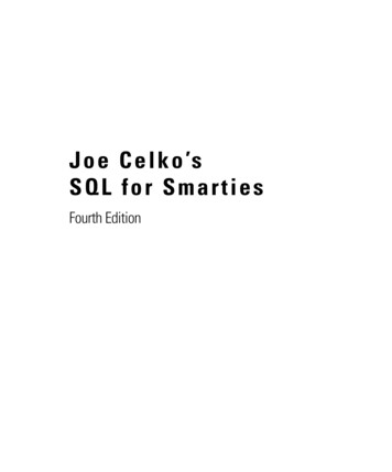
A Baseline Strategy: Optimized Submit-and-LeaveShortfall vs. Limit Pricedeep in OBM.O. at startRisk vs. Limit PriceEfficient Frontier[Nevmyvaka, K., Papandreou, Sycara IEEE CEC 2005]
Private State Variables Only: Time and Inventory RemainingAverage Improvement Over Optimized Submit-and-LeaveT 4 I 127.16%T 8 I 131.15%T 4 I 430.99%T 8 I 434.90%T 4 I 831.59%T 8 I 835.50%
Improvement From Order Book FeaturesBid Volume-0.06% Ask Volume-0.28%Bid-Ask Volume Misbalance0.13% Bid-Ask Spread7.97%Price Level0.26% Immediate Market Order Cost4.26%Signed Transaction Volume2.81% Price Volatility-0.55%Spread Volatility1.89% Signed Incoming VolumeSpread Immediate Cost8.69% Spread ImmCost Signed Vol0.59%12.85%
Microstructure and Market-Making Canonical market-making:–––– A simple model, algorithm and result:––––––– always maintain outstanding buy & sell limit orders; can adjust spreadif a buy-sell pair executed, earn the spreadonly one side executed: accumulation of risk/inventorymay have to liquidate inventory at a loss at market closeprice time series p 0, ,p T, where d t p {t 1} – p t D, infinite liquidityalgorithm maintains ladder of matched order pairs up to depth Dlet z p T – p 0 (global price change) and K \sum t d t (sum of local changes)then profit K – z 2 /-1 random walk (Brownian): profit 0but profit 0 on any “mean-reverting” time series[Chakraborty and K., ACM EC 2011]Learning and market-making: Sanmay Das and colleagues
Outline I. Market Microstructure and Optimized Execution– online algorithms and competitive analysis– reinforcement learning for optimized execution– microstructure and market-making II. Mechanism Innovation: a Case Study– difficult trades and dark pools– the order dispersion problem– censoring, exploration, and exploitation III. No-Regret Learning, Portfolio Optimization, and Risk––––no-regret learning and financetheoretical guarantees and empirical performanceincorporating risk: Sharpe ratio, mean-variance, market benchmarksno-regret and option pricing
Modern “Light” ExchangesMajor disadvantage: executing very large orders* distributing over time and venues insufficient* many buy-side parties are “compelled”Thus the advent of Dark Pools* specify side and volume only* no price, execution by time priority* price generally pegged to light midpoint* not seeking price improvement, just execution* only learn (partial) fill for your order
TORA CrosspointInstinetSmartPoolPosit/MatchNow from Investment Technology Group (ITG)LiquidnetNYFIX MillenniumPulse Trading BlockCrossRiverCrossPipeline Trading SystemsBarclays Capital - LX Liquidity CrossBNP ParibasBNY ConvergEx GroupCiti - Citi MatchCredit Suisse - CrossFinderFidelity Capital MarketsGETCO - GETMatchedGoldman Sachs SIGMA XKnight Capital Group - Knight Link, Knight MatchDeutsche Bank Global Markets - DBA(Europe), SuperX ATS (US)Merrill Lynch – MLXNMorgan StanleyNomura - Nomura NXUBS Investment BankBallista ATS Ballista Securities LLCBlocSec[citation needed]Bloomberg Tradebook (an affiliate of Bloomberg L.P.)Daiwa – DRECTBIDS Trading - BIDS ATSLeveL ATSInternational Securities ExchangeNYSE EuronextBATS TradingDirect EdgeSwiss BlockNordic@MidChi-XTurquoiseBloomberg TradebookFidessa - SpotlightSuperX – Deutsche BankASOR – Quod FinancialProgress ApamaONEPIPE – Weeden & Co. & Pragma FinancialXasax CorporationCrossfire – Credit Agricole Cheuvreux
The Dark Pool (Allocation) ProblemGiven a sequence or distribution of “client” or parent orders, how should wedistribute the desired volumes over a large number of dark pools?(a.k.a. Smart Order Routing (SOR))May initially know little about relative quality/properties of pools* may be specific to name, volatility, volume, * a learning problem* (related to “newsvendor problem” from OR)To simplify things, will generally assume:* client orders all on one side (e.g. selling)* client orders come i.i.d. from a fixed distribution even though our “child” submissions to pools will not be i.i.d.* statistical properties of a given pool are staticAll can be relaxed in various ways, at the cost of complexity
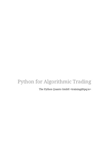
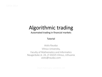
probabilityModeling Available Volume: Single PoolP[s]shares availablev shares submitteddraw s Pexecute min(v,s)censored observations
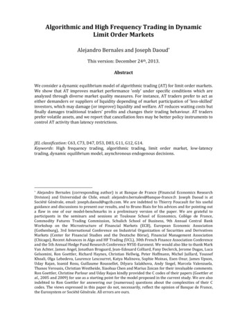
Pool 1Multiple PoolsPool 2v2 sharesClient volume VPool 3Allocate How?Pool 4
A Statistical Sub-ProblemFrom a given pool P[s], we observe a sequence of censored executionsAt time t, we submitted v(t) shares and s(t) v(t) were executedQ: What is the maximum likelihood estimate of P[s]?A: The Kaplan-Meier estimator from biostatistics and survival analysis* start with empirical distribution of uncensored observations* process censored observations from largest to smallest* distribute over larger values proportional to their current weightKnown to converge to P[s] asymptotically under i.i.d. submissions* also need support conditions on submission distribution* for us, i.i.d. violated by dependence between venue submissionsCan prove and use a stronger lemma (paraphrased):* for any volume s, P[s] – P’[s] 1/sqrt(N(s))* N(s) number of times we have submitted s sharesFor analysis only, define a cut-off c[i] for each venue distribution P i:* we “know” P i[s] accurately for s c[i]* may know little or nothing above c[i]
The Learning Algorithm and Analysis[Ganchev, K., Nevmyvaka, Wortman UAI, CACM]Algorithm:initialize estimated distributions P’ 1, P’ 2, , P’ krepeat:* compute greedy optimal allocations to each venue given the P’ i* use censored executions to re-estimate P’ i using optimistic K-MAnalysis:* if allocation to every venue i is c[i], already near-optimal;know “enough” about the P i to make this allocation (“exploit”)* if for some venue j, submitted volume c[j], we “explore”;so eventually c[j] will increase improve P’ j* optimistic: slight tail modification ensures always exploit/explore* analogy to E 3/RMAX family for RLMain Theorem: algorithm efficiently converges to near-optimal* non-parametric and parametric versions
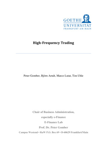
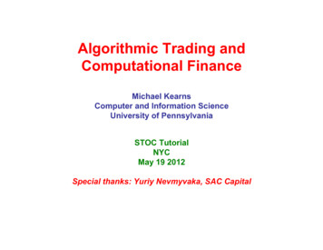
Algorithm vs. Uniform Allocation
Algorithm vs. Ideal Allocation
Algorithm vs. Bandits** Nice no-regret follow-up: Agarwal, Barlett, Dama AISTATS 2010
Outline I. Market Microstructure and Optimized Execution– online algorithms and competitive analysis– reinforcement learning for optimized execution– microstructure and market-making II. Mechanism Innovation: a Case Study– difficult trades and dark pools– the order dispersion problem– censoring, exploration, and exploitation III. No-Regret Learning, Portfolio Optimization, and Risk––––no-regret learning and financetheoretical guarantees and empirical performanceincorporating risk: Sharpe ratio, mean-variance, market benchmarksno-regret and option pricing
Basic Framework An underlying universe of K assets U {S 1, ,S K}Goal: manage a “profitable” portfolio over U– each trading period S i grows/shrinks q i (1 r i), r i in [-1,infinity]– we maintain a distribution w of wealth, fraction w i in S i– all quantities indexed (superscripted) by time t Traditionally: K assets are long positions in common stocksMore generally: K assets are any collection of investment instruments:– long and short positions in common stocks, cash, futures, derivatives– technical trading strategies, pairs strategies, etc.– generally need instruments/performance to be “stateless”: can be entered at any time How do we measure performance relative to U?– average return ( “the market”): place 1/K of initial wealth in each S i and leave it there– Uniform Constant Rebalanced Portfolio (UCRP): set w i 1/K and rebalance every period exponential growth (factor 9/8) on S 1 (1,1,1,1,1 .) and S 2 (2,1/2,2,1/2, ); reversion effect– Best Single Stock (BSS) in hindsight– Best Constant Rebalanced Portfolio (BCRP) in hindsight– Note: must place some restrictions on comparison class
Online Algorithms: Theory Assume nothing about sequence of returns r i (except maybe max loss)On arbitrary sequence r 1, r T, algorithm A dynamically adjusts portfolio w 1, ,w tCompare cumulative return of A to BSS or BCRP (in hindsight)Powerful families of no-regret algorithms: for all sequences,––– Return(A)/T Return(BSS)/T – O(sqrt(log(K)/T))or log(A’s wealth)/T log(BCRP wealth)/T – O(K/T) (Cover’s algorithm; exponential growth)“complexity penalty” for large K; per-step regret is vanishing with THow is this possible?–note: for this to be interesting, need BSS or BCRP to strongly outperform the average
Cover’s Algorithm K stocks, T periodsW t(p) wealth of portfolio/distribution p after t periodsInvest initial wealth uniformly across all CRPs and leave itEquivalent:–– Learning at the stock level, but not at the portfolio level!Now let p* maximize W(p*) W T(p*) (BCRP in hindsight)Then for any c: W(A) r K (1-r) T W(p*)–– initial portfolio p 1 (1/K, ,1/K)p {t 1} \integral {p} W t(p)p dp/\integral {p} W t(p) dpr K: amount of weight in r-ball around p*(1-r) T: if p is within r of p*, must make at worst factor (1-r) less at each periodPicking r 1/T: W(A) (1/T) K (1 – 1/T) T W(p*) (1/T) K W(p*)So log W(A) log W(p*) – K log TOnly interesting for exponential growth
Tractable Algorithms Most update weights multiplicatively, not additivelyFlavor of a typical algorithm (e.g. Exponential Weights):– One (crucial) parameter: learning rate η–––– w i exp(η*r i)w i, renormalizefor the theory, need to optimize η 1/sqrt(T)generally are assuming momentum rather than mean reversionnote: η 0 (no learning) is UCRP; a form of mean reversionvalue of η also strongly influences portfolio concentration variance/riskLet’s look at some empirical performance
Data Period: early 2005 – end 2011 ( 7 years)Underlying Instruments: stocks in S&P 500 (selection bias)Daily (closing) returnsWealth of investing 1 in each stock
long positions onlyUCRP: magentaCover’s algorithm: redExponential Weights (optimized): green
long and short positionUCRP long only: magentaUCRP short only: yellowCover’s algorithm: redExponential Weights: green
What About Risk? Sharpe Ratio (mean of returns)/(standard deviation of returns)Mean-Variance (MV) criterion mean – varianceMaximum Drawdown; Value at Risk (VaR)Concentration limitsMarket index/average as a lower bound
Some Relevant Theory What about no regret compared to BSS in hindsight w.r.t. risk-return metrics?––––– But can preserve traditional no-regret with benchmarking to average––––– e.g. BSS Sharpe, BSS M-V, can prove any online algorithm must have constant regret in fact, even offline competitive ratio must be constantvariance constraints introduce switching costs or state[Even-Dar, K., Wortman ALT 2006]additive reward settingguarantee O(sqrt(T)) cumulative regret to best, O(1) to averageIdea: only increase η as data “proves” best will beat averageworst case: track the market[Even-Dar, K, Mansour, Wortman COLT 2007]“State” generally ruins no-regret theoryLots of room for innovation/improvement
No-Regret and Option Pricing Option (European call): right, but not obligation, to purchase shares at a fixedprice and future timeE.g. AAPL now trading 546; option to purchase at 600 in a yearOption should cost something --- but what?– Black-Scholes:–––– hedging strategy that has no regret to option payoffmultiplicative weight update algorithmAbernethy, Frongillo, Wibisono STOC 2012:–– assume future price evolution follows geometric Brownian motionB: borrow money to buy options now; if options “in the money”, exercise and pay back loanS: sell options now for cash; if options in the money, pay counterpartycorrect option price: neither B nor S has positive expected profitWhat if the future price evolution is arbitrary?DeMarzo, Kremer, Mansour STOC 06:–– depends on uncertainty/fluctuationsview option pricing as an adversarial gameminimax price is same as Black-Sholes under Brownian motion!More complex derivatives with asymmetric info may be intractable to price–––“pay 1 if AAPL price increases x% where x matches last two digits of a prime factor of N”intractability of planted dense subgraph difficulty in pricing natural derivatives (e.g. CDS)Arora, Barak, Brunnermeier, Ge
Conclusions Many algorithmic challenges in modern financeLower level: market microstructure, optimized execution metrics & problemsHigher level: portfolio optimization, option pricing, no-regret algorithmsNew market mechanisms lead to new algorithmic challenges (e.g. dark pools)
Algorithmic Trading and Computational Finance . STOC Tutorial NYC May 19 2012 Special thanks: Yuriy Nevmyvaka, SAC Capital . Takeaways There are many interesting and challenging algorithmic and modeling problems in “traditional” financial markets .