Transcription
Chapter 6Power SeriesPower series are one of the most useful type of series in analysis. For example,we can use them to define transcendental functions such as the exponential andtrigonometric functions (and many other less familiar functions).6.1. IntroductionA power series (centered at 0) is a series of the form an xn a0 a1 x a2 x2 · · · an xn . . . .n 0where the an are some coefficients. If all but finitely many of the an are zero,then the power series is a polynomial function, but if infinitely many of the an arenonzero, then we need to consider the convergence of the power series.The basic facts are these: Every power series has a radius of convergence 0 R , which depends on the coefficients an . The power series converges absolutelyin x R and diverges in x R, and the convergence is uniform on every interval x ρ where 0 ρ R. If R 0, the sum of the power series is infinitelydifferentiable in x R, and its derivatives are given by differentiating the originalpower series term-by-term.Power series work just as well for complex numbers as real numbers, and arein fact best viewed from that perspective, but we restrict our attention here toreal-valued power series.Definition 6.1. Let (an ) n 0 be a sequence of real numbers and c R. The powerseries centered at c with coefficients an is the series an (x c)n .n 073
746. Power SeriesHere are some power series centered at 0: xn 1 x x2 x3 x4 . . . ,n 0 1 n111x 1 x x2 x3 x4 . . . ,n!2624n 0 n 0 (n!)xn 1 x 2x2 6x3 24x4 . . . ,n( 1)n x2 x x2 x4 x8 . . . ;n 0and here is a power series centered at 1: ( 1)n 1111(x 1)n (x 1) (x 1)2 (x 1)3 (x 1)4 . . . .n234n 1The power series in Definition 6.1 is a formal expression, since we have not saidanything about its convergence. By changing variables x 7 (x c), we can assumewithout loss of generality that a power series is centered at 0, and we will do sowhen it’s convenient.6.2. Radius of convergenceFirst, we prove that every power series has a radius of convergence.Theorem 6.2. Let an (x c)nn 0be a power series. There is an 0 R such that the series converges absolutelyfor 0 x c R and diverges for x c R. Furthermore, if 0 ρ R, thenthe power series converges uniformly on the interval x c ρ, and the sum of theseries is continuous in x c R.Proof. Assume without loss of generality that c 0 (otherwise, replace x by x c).Suppose the power series an xn0n 0converges for some x0 R with x0 ̸ 0. Then its terms converge to zero, so theyare bounded and there exists M 0 such that an xn0 Mfor n 0, 1, 2, . . . .If x x0 , then an xn an xn0 xx0n M rn ,r x 1.x0 Comparingthe power series with the convergent geometric seriesM rn , we see thatan xn is absolutely convergent. Thus, if the power series converges for somex0 R, then it converges absolutely for every x R with x x0 .
6.2. Radius of convergenceLet75{} R sup x 0 :an xn converges .If R 0, then the series converges only for x 0. If R 0, then the seriesconverges absolutely for every x R with x R, because it converges for somex0 R with x x0 R. Moreover, the definition of R implies that the seriesdiverges for every x R with x R. If R , then the series converges for allx R.Finally,let 0 ρ R and suppose x ρ. Choose σ 0 such that ρ σ R. Then an σ n converges, so an σ n M , and thereforex nρ n an σ n M rn , an xn an σ n σσ where r ρ/σ 1. SinceM rn , the M -test (Theorem 5.22) implies thatthe series converges uniformly on x ρ, and then it follows from Theorem 5.16that the sum is continuous on x ρ. Since this holds for every 0 ρ R, thesum is continuous in x R. The following definition therefore makes sense for every power series.Definition 6.3. If the power series an (x c)nn 0converges for x c R and diverges for x c R, then 0 R is calledthe radius of convergence of the power series.Theorem 6.2 does not say what happens at the endpoints x c R, and ingeneral the power series may converge or diverge there. We refer to the set of allpoints where the power series converges as its interval of convergence, which is oneof(c R, c R), (c R, c R], [c R, c R), [c R, c R].We will not discuss any general theorems about the convergence of power series atthe endpoints (e.g. the Abel theorem).Theorem 6.2 does not give an explicit expression for the radius of convergenceof a power series in terms of its coefficients. The ratio test gives a simple, but useful,way to compute the radius of convergence, although it doesn’t apply to every powerseries.Theorem 6.4. Suppose that an ̸ 0 for all sufficiently large n and the limitR limn anan 1exists or diverges to infinity. Then the power series n 0has radius of convergence R.an (x c)n
766. Power SeriesProof. Letan 1 (x c)n 1an 1 x c lim.nn n an (x c)anBy the ratio test, the power series converges if 0 r 1, or x c R, anddiverges if 1 r , or x c R, which proves the result. r limThe root test gives an expression for the radius of convergence of a generalpower series.Theorem 6.5 (Hadamard). The radius of convergence R of the power series an (x c)nn 0is given by1R 1/nlim supn an where R 0 if the lim sup diverges to , and R if the lim sup is 0.Proof. Let1/nr lim sup an (x c)n n x c lim sup an 1/n.n By the root test, the series converges if 0 r 1, or x c R, and diverges if1 r , or x c R, which proves the result. This theorem provides an alternate proof of Theorem 6.2 from the root test; infact, our proof of Theorem 6.2 is more-or-less a proof of the root test.6.3. Examples of power seriesWe consider a number of examples of power series and their radii of convergence.Example 6.6. The geometric series xn 1 x x2 . . .n 0has radius of convergence1 1.1so it converges for x 1, to 1/(1 x), and diverges for x 1. At x 1, theseries becomes1 1 1 1 .and at x 1 it becomesR limn 1 1 1 1 1 .,so the series diverges at both endpoints x 1. Thus, the interval of convergenceof the power series is ( 1, 1). The series converges uniformly on [ ρ, ρ] for every0 ρ 1 but does not converge uniformly on ( 1, 1) (see Example 5.20. Notethat although the function 1/(1 x) is well-defined for all x ̸ 1, the power seriesonly converges to it when x 1.
6.3. Examples of power series77Example 6.7. The series 1 n111x x x2 x3 x4 . . .n234n 1has radius of convergence()11/n lim 1 1.n 1/(n 1)n nR limAt x 1, the series becomes the harmonic series 1 1 11 1 .,n2 3 4n 1which diverges, and at x 1 it is minus the alternating harmonic series 1 1 1( 1)n 1 . . . ,n2 3 4n 1which converges, but not absolutely. Thus the interval of convergence of the powerseries is [ 1, 1). The series converges uniformly on [ ρ, ρ] for every 0 ρ 1 butdoes not converge uniformly on ( 1, 1).Example 6.8. The power series 1 n11x 1 x x x3 . . .n!2!3!n 0has radius of convergenceR limn 1/n!(n 1)! lim lim (n 1) ,n n 1/(n 1)!n!so it converges for all x R. Its sum provides a definition of the exponentialfunction exp : R R. (See Section 6.5.)Example 6.9. The power series 11( 1)n 2nx 1 x2 x4 . . .(2n)!2!4!n 0has radius of convergence R , and it converges for all x R. Its sum providesa definition of the cosine function cos : R R.Example 6.10. The series ( 1)nn 0 (2n 1)!x2n 1 x 1 31x x5 . . .3!5!has radius of convergence R , and it converges for all x R. Its sum providesa definition of the sine function sin : R R.Example 6.11. The power series n 0(n!)xn 1 x (2!)x (3!)x3 (4!)x4 . . .
786. Power Series0.60.5y0.40.30.20.1000.20.40.60.81x n 2n on [0, 1).Figure 1. Graph of the lacunary power series y n 0 ( 1) xIt appears relatively well-behaved; however, the small oscillations visible nearx 1 are not a numerical artifact.has radius of convergencen!1 lim 0,n (n 1)!n n 1R limso it converges only for x 0. If x ̸ 0, its terms grow larger once n 1/ x and (n!)xn as n .Example 6.12. The series 11( 1)n 1(x 1)n (x 1) (x 1)2 (x 1)3 . . .n23n 1has radius of convergenceR limn ( 1)n 1 /nn1 lim lim 1,n 2n n 1n 1 1/n( 1)/(n 1)so it converges if x 1 1 and diverges if x 1 1. At the endpoint x 2, thepower series becomes the alternating harmonic series1 1 11 .,2 3 4which converges. At the endpoint x 0, the power series becomes the harmonicseries1 1 11 .,2 3 4which diverges. Thus, the interval of convergence is (0, 2].
6.4. Differentiation of power series79Example 6.13. The power series n( 1)n x2 x x2 x4 x8 x16 x32 . . .n 0{withan 1 if n 2k ,0 if n ̸ 2k ,has radius of convergence R 1. To prove this, note that theconverges for series x 1 by comparison with the convergent geometric series x n , since{ x nif n 2k ,n an x n0 x if n ̸ 2k .If x 1, the terms do not approach 0 as n , so the series diverges. Alternatively, we have{1 if n 2k ,1/n an 0 if n ̸ 2k ,solim sup an 1/n 1n and the root test (Theorem 6.5) gives R 1. The series does not converge at eitherendpoint x 1, so its interval of convergence is ( 1, 1).There are successively longer gaps (or “lacuna”) between the powers with nonzero coefficients. Such series are called lacunary power series, and they have manyinteresting properties. For example, although the series does not converge at x 1,one can ask if[ ] nlim ( 1)n x2x 1n 0exists. In a plot of this sum on [0, 1), shown in Figure 1, the function appearsrelatively well-behaved near x 1. However, Hardy (1907) proved that the functionhas infinitely many, very small oscillations as x 1 , as illustrated in Figure 2,and the limit does not exist. Subsequent results by Hardy and Littlewood (1926)showed, under suitable assumptions on the growth of the “gaps” between non-zerocoefficients, that if the limit of a lacunary power series as x 1 exists, then theseries must converge at x 1. Since the lacunary power series considered here doesnot converge at 1, its limit as x 1 cannot exist6.4. Differentiation of power seriesWe saw in Section 5.4.3 that, in general, one cannot differentiate a uniformly convergent sequence or series. We can, however, differentiate power series, and theybehaves as nicely as one can imagine in this respect. The sum of a power seriesf (x) a0 a1 x a2 x2 a3 x3 a4 x4 . . .is infinitely differentiable inside its interval of convergence, and its derivativef ′ (x) a1 2a2 x 3a3 x2 4a4 x3 . . .
806. Power 810.490.990.9920.994x0.9960.9981x n 2n near x 1,Figure 2. Details of the lacunary power seriesn 0 ( 1) xshowing its oscillatory behavior and the nonexistence of a limit as x 1 .is given by term-by-term differentiation. To prove this, we first show that theterm-by-term derivative of a power series has the same radius of convergence as theoriginal power series. The idea is that the geometrical decay of the terms of thepower series inside its radius of convergence dominates the algebraic growth of thefactor n.Theorem 6.14. Suppose that the power series an (x c)nn 0has radius of convergence R. Then the power series nan (x c)n 1n 1also has radius of convergence R.Proof. Assume without loss of generality that c 0, and suppose x R. Chooseρ such that x ρ R, and let x ,0 r 1.ρTo estimate the terms in the differentiated power series by the terms in the originalseries, we rewrite their absolute values as follows:( )n 1nrn 1n x an ρn an ρn .nan xn 1 ρ ρρ n 1The ratio test shows that the seriesnrconverges, since[][() ]n(n 1)r1lim lim1 r r 1,n n nrn 1nr so the sequence (nrn 1 ) is bounded, by M say. It follows thatnan xn 1 M an ρn ρfor all n N.
6.4. Differentiation of power series81 The series an ρn converges, since ρ R, so the comparison test implies that n 1nan xconverges absolutely. Conversely, suppose x R. Then an xn diverges (sincean xn diverges)and1nan xn 1 an xn x for n 1, so the comparison test implies thatnan xn 1 diverges. Thus the serieshave the same radius of convergence. Theorem 6.15. Suppose that the power seriesf (x) an (x c)nfor x c Rn 0has radius of convergence R 0 and sum f . Then f is differentiable in x c Rand f ′ (x) nan (x c)n 1for x c R.n 1Proof. The term-by-term differentiated power series converges in x c R byTheorem 6.14. We denote its sum byg(x) nan (x c)n 1 .n 1Let 0 ρ R. Then, by Theorem 6.2, the power series for f and g both convergeuniformly in x c ρ. Applying Theorem 5.18 to their partial sums, we concludethat f is differentiable in x c ρ and f ′ g. Since this holds for every0 ρ R, it follows that f is differentiable in x c R and f ′ g, which provesthe result. Repeated application Theorem 6.15 implies that the sum of a power series isinfinitely differentiable inside its interval of convergence and its derivatives are givenby term-by-term differentiation of the power series. Furthermore, we can get anexpression for the coefficients an in terms of the function f ; they are simply theTaylor coefficients of f at c.Theorem 6.16. If the power seriesf (x) an (x c)nn 0has radius of convergence R 0, then f is infinitely differentiable in x c Randf (n) (c)an .n!Proof. We assume c 0 without loss of generality. Applying Theorem 6.16 to thepower seriesf (x) a0 a1 x a2 x2 a3 x3 · · · an xn . . .
826. Power Seriesk times, we find that f has derivatives of every order in x R, andf ′ (x) a1 2a2 x 3a3 x2 · · · nan xn 1 . . . ,f ′′ (x) 2a2 (3 · 2)a3 x · · · n(n 1)an xn 2 . . . ,f ′′′ (x) (3 · 2 · 1)a3 · · · n(n 1)(n 2)an xn 3 . . . ,.f (k) (x) (k!)ak · · · n!xn k . . . ,(n k)!where all of these power series have radius of convergence R. Setting x 0 in theseseries, we getf (k) (0),a0 f (0), a1 f ′ (0), . . . ak k!which proves the result (after replacing 0 by c). One consequence of this result is that convergent power series with differentcoefficients cannot converge to the same sum.Corollary 6.17. If two power series an (x c)n ,n 0 bn (x c)nn 0have nonzero-radius of convergence and are equal on some neighborhood of 0, thenan bn for every n 0, 1, 2, . . . .Proof. If the common sum in x c δ is f (x), we havef (n) (c)f (n) (c),bn ,n!n!since the derivatives of f at c are determined by the values of f in an arbitrarilysmall open interval about c, so the coefficients are equal an 6.5. The exponential functionWe showed in Example 6.8 that the power series111E(x) 1 x x2 x3 · · · xn . . . .2!3!n!has radius of convergence . It therefore defines an infinitely differentiable functionE : R R.Term-by-term differentiation of the power series, which is justified by Theorem 6.15, implies that11E ′ (x) 1 x x2 · · · x(n 1) . . . ,2!(n 1)!so E ′ E. Moreover E(0) 1. As we show below, there is a unique functionwith these properties, and they are shared by the exponential function ex . Thus,this power series provides an analytical definition of ex E(x). All of the other
6.5. The exponential function83familiar properties of the exponential follow from its power-series definition, andwe will prove a few of them.First, we show that ex ey ex y . We continue to write the function as E(x) toemphasise that we use nothing beyond its power series definition.Proposition 6.18. For every x, y R,E(x)E(y) E(x y).Proof. We haveE(x) xjj 0j!,E(y) ykk 0k!.Multiplying these series term-by-term and rearranging the sum, which is justifiedby the absolute converge of the power series, we getE(x)E(y) xj y kj 0 k 0 n n 0 k 0j! k!xn k y k.(n k)! k!From the binomial theorem,nn xn k y k1 n!1n xn k y k (x y) .(n k)! k!n!(n k)! k!n!k 0k 0Hence,E(x)E(y) (x y)n E(x y),n!n 0 which proves the result.In particular, it follows thatE( x) 1.E(x)Note that E(x) 0 for all x 0 since all the terms in its power series are positive,so E(x) 0 for every x R.The following proposition, which we use below in Section 6.6.2, states that exgrows faster than any power of x as x .Proposition 6.19. Suppose that n is a non-negative integer. Thenxn 0.x E(x)limProof. The terms in the power series of E(x) are positive for x 0, so for everyk N xkxn for all x 0.E(x) n!k!n 0
846. Power SeriesTaking k n 1, we get for x 0 that0 xnxn(n 1)! (n 1) .E(x)xx/(n 1)!Since 1/x 0 as x , the result follows. Finally, we prove that the exponential is characterized by the properties E ′ Eand E(0) 1. This is a uniqueness result for an initial value problem for a simplelinear ordinary differential equation.Proposition 6.20. Suppose f : R R is a differentiable function such thatf ′ f,f (0) 1.Then f E.Proof. Suppose that f ′ f . Then using the equation E ′ E, the fact that E isnonzero on R, and the quotient rule, we get( )′f E ′ Ef ′f E Eff 0.EE2E2It follows from Theorem 4.29 that f /E is constant on R. Since f (0) E(0) 1,we have f /E 1, which implies that f E. The logarithm can be defined as the inverse of the exponential. Other transcendental functions, such as the trigonometric functions, can be defined in termsof their power series, and these can be used to prove their usual properties. Wewill not do this in detail; we just want to emphasize that, once we have developedthe theory of power series, we can define all of the functions arising in elementarycalculus from the first principles of analysis.6.6. Taylor’s theorem and power seriesTheorem 6.16 looks similar to Taylor’s theorem, Theorem 4.41. There is, however, afundamental difference. Taylor’s theorem gives an expression for the error betweena function and its Taylor polynomial of degree n. No questions of convergence areinvolved here. On the other hand, Theorem 6.16 asserts the convergence of aninfinite power series to a function f , and gives an expression for the coefficients ofthe power series in terms of f . The coefficients of the Taylor polynomials and thepower series are the same in both cases, but the Theorems are different.Roughly speaking, Taylor’s theorem describes the behavior of the Taylor polynomials Pn (x) of f as x c with n fixed, while the power series theorem describesthe behavior of Pn (x) as n with x fixed.6.6.1. Smooth functions and analytic functions. To explain the differencebetween Taylor’s theorem and power series in more detail, we introduce an important distinction between smooth and analytic functions: smooth functions havecontinuous derivatives of all orders, while analytic functions are sums of powerseries.
6.6. Taylor’s theorem and power series85Definition 6.21. Let k N. A function f : (a, b) R is C k on (a, b), writtenf C k (a, b), if it has continuous derivatives f (j) : (a, b) R of orders 1 j k.A function f is smooth (or C , or infinitely differentiable) on (a, b), written f C (a, b), if it has continuous derivatives of all orders on (a, b).In fact, if f has derivatives of all orders, then they are automatically continuous,since the differentiability of f (k) implies its continuity; on the other hand, theexistence of k derivatives of f does not imply the continuity of f (k) . The statement“f is smooth” is sometimes used rather loosely to mean “f has as many continuousderivatives as we want,” but we will use it to mean that f is C .Definition 6.22. A function f : (a, b) R is analytic on (a, b) if for every c (a, b)f is the sum in a neighborhood of c of a power series centered at c with nonzeroradius of convergence.Strictly speaking, this is the definition of a real analytic function, and analyticfunctions are complex functions that are sums of power series. Since we consideronly real functions, we abbreviate “real analytic” to “analytic.”Theorem 6.16 implies that an analytic function is smooth: If f is analytic on(a, b) and c (a, b), then there is an R 0 and coefficients (an ) such thatf (x) an (x c)nfor x c R.n 0Then Theorem 6.16 implies that f has derivatives of all orders in x c R, andsince c (a, b) is arbitrary, f has derivatives of all orders in (a, b). Moreover, itfollows that the coefficients an in the power series expansion of f at c are given byTaylor’s formula.What is less obvious is that a smooth function need not be analytic. If f issmooth, then we can define its Taylor coefficients an f (n) (c)/n! at c for everyn 0, and write down the corresponding Taylor seriesan (x c)n . The problemis that the Taylor series may have zero radius of convergence, in which case itdiverges for every x ̸ c, or the power series may converge, but not to f .6.6.2. A smooth, non-analytic function. In this section, we give an exampleof a smooth function that is not the sum of its Taylor series.It follows from Proposition 6.19 that ifp(x) n ak xkk 0is any polynomial function, thenp(x) xklim alim 0.kx exx exnk 0We will use this limit to exhibit a non-zero function that approaches zero fasterthan every power of x as x 0. As a result, all of its derivatives at 0 vanish, eventhough the function itself does not vanish in any neighborhood of 0. (See Figure 3.)
866. Power Series 50.950.84.5x 1040.73.50.63yy0.52.50.420.31.50.210.10 10.5012x3450 0.0200.020.04x0.060.080.1Figure 3. Left: Plot y ϕ(x) of the smooth, non-analytic function definedin Proposition 6.23. Right: A detail of the function near x 0. The dottedline is the power-function y x6 /50. The graph of ϕ near 0 is “flatter’ thanthe graph of the power-function, illustrating that ϕ(x) goes to zero faster thanany power of x as x 0.Proposition 6.23. Define ϕ : R R by{exp( 1/x) if x 0,ϕ(x) 0if x 0.Then ϕ has derivatives of all orders on R andϕ(n) (0) 0for all n 0.Proof. The infinite differentiability of ϕ(x) at x ̸ 0 follows from the chain rule.Moreover, its nth derivative has the form{pn (1/x) exp( 1/x) if x 0,(n)ϕ (x) 0if x 0,where pn (1/x) is a polynomial in 1/x. (This follows, for example, by induction.)Thus, we just have to show that ϕ has derivatives of all orders at 0, and that thesederivatives are equal to zero.First, consider ϕ′ (0). The left derivative ϕ′ (0 ) of ϕ at 0 is clearly 0 sinceϕ(0) 0 and ϕ(h) 0 for all h 0. For the right derivative, writing 1/h x andusing Proposition 6.19, we get][ϕ(h) ϕ(0)ϕ′ (0 ) lim hh 0exp( 1/h) limhh 0 x lim xx e 0.Since both the left and right derivatives equal zero, we have ϕ′ (0) 0.To show that all the derivatives of ϕ at 0 exist and are zero, we use a proofby induction. Suppose that ϕ(n) (0) 0, which we have verified for n 1. The
6.6. Taylor’s theorem and power series87left derivative ϕ(n 1) (0 ) is clearly zero, so we just need to prove that the rightderivative is zero. Using the form of ϕ(n) (h) for h 0 and Proposition 6.19, we getthat[ (n)]ϕ (h) ϕ(n) (0)(n 1) ϕ(0 ) lim hh 0pn (1/h) exp( 1/h) lim hh 0xpn (x) limx ex 0, which proves the result.Corollary 6.24. The function ϕ : R R defined by{exp( 1/x) if x 0,ϕ(x) 0if x 0,is smooth but not analytic on R.Proof. From Proposition 6.23, the function ϕ is smooth, and the nth Taylor coefficient of ϕ at 0 is an 0. The Taylor series of ϕ at 0 therefore converges to 0, soits sum is not equal to ϕ in any neighborhood of 0, meaning that ϕ is not analyticat 0. The fact that the Taylor polynomial of ϕ at 0 is zero for every degree n N doesnot contradict Taylor’s theorem, which states that for x 0 there exists 0 ξ xsuch thatpn 1 (1/ξ) 1/ξ n 1ϕ(x) ex.(n 1)!Since the derivatives of ϕ are bounded, this shows that for every n N there existsa constant Cn 1 such that0 ϕ(x) Cn 1 xn 1for all 0 x ,but this does not imply that ϕ(x) 0.We can construct other smooth, non-analytic functions from ϕ.Example 6.25. The functionψ(x) {exp( 1/x2 ) if x ̸ 0,0if x 0,is infinitely differentiable on R, since ψ(x) ϕ(x2 ) is a composition of smoothfunctions.The following example is useful in many parts of analysis.Definition 6.26. A function f : R R has compact support if there exists R 0such that f (x) 0 for all x R with x R.
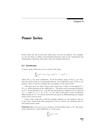
886. Power Series0.40.350.3y0.250.20.150.10.050 2 1.5 1 0.50x0.511.52Figure 4. Plot of the smooth, compactly supported “bump” function definedin Example 6.27.It isn’t hard to construct continuous functions with compact support; one example that vanishes for x 1 is{1 x if x 1,f (x) 0if x 1.By matching left and right derivatives of a piecewise-polynomial function, we cansimilarly construct C 1 or C k functions with compact support. Using ϕ, however,we can construct a smooth (C ) function with compact support, which might seemunexpected at first sight.Example 6.27. The function{exp[ 1/(1 x2 )] if x 1,η(x) 0if x 1,is infinitely differentiable on R, since η(x) ϕ(1 x2 ) is a composition of smoothfunctions. Moreover, it vanishes for x 1, so it is a smooth function with compactsupport. Figure 4 shows its graph.The function ϕ defined in Proposition 6.23 illustrates that knowing the valuesof a smooth function and all of its derivatives at one point does not tell us anythingabout the values of the function at other points. By contrast, an analytic functionon an interval has the remarkable property that the value of the function and all ofits derivatives at one point of the interval determine its values at all other points
6.7. Appendix: Review of series89of the interval, since we can extend the function from point to point by summingits power series. (This claim requires a proof, which we omit.)For example, it is impossible to construct an analytic function with compactsupport, since if an analytic function on R vanishes in any interval (a, b) R, thenit must be identically zero on R. Thus, the non-analyticity of the “bump”-functionη in Example 6.27 is essential.6.7. Appendix: Review of seriesWe summarize the results and convergence tests that we use to study power series.Power series are closely related to geometric series, so most of the tests involvecomparisons with a geometric series.Definition 6.28. Let (an ) be a sequence of real numbers. The series ann 1converges to a sum S R if the sequence (Sn ) of partial sumsSn n akk 1converges to S. The series converges absolutely if an n 1converges.The following Cauchy condition for series is an immediate consequence of theCauchy condition for the sequence of partial sums.Theorem 6.29 (Cauchy condition). The series ann 1converges if and only for every ϵ 0 there exists N N such thatn ak am 1 am 2 · · · an ϵfor all n m N .k m 1Proof. The series converges if and only if the sequence (Sn ) of partial sums isCauchy, meaning that for every ϵ 0 there exists N such that Sn Sm n ak ϵfor all n m N ,k m 1which proves the result.
906. Power SeriesSincen n ak k m 1 ak k m 1 the seriesan is Cauchy if an is Cauchy, so an absolutely convergent seriesconverges. We have the following necessary, but not sufficient, condition for convergence of a series.Theorem 6.30. If the series ann 1converges, thenlim an 0.n Proof. If the series converges, then it is Cauchy. Taking m n 1 in the Cauchycondition in Theorem 6.29, we find that for every ϵ 0 there exists N N such that an ϵ for all n N , which proves that an 0 as n .Next, we derive the comparison, ratio, and root tests, which provide explicitsufficient conditions for the convergence of a series. Theoreman converges. 6.31 (Comparison test). Suppose that bn an andThenbn converges absolutely. Proof. Sincean converges it satisfies the Cauchy condition, and sincenn bk akthe seriesabsolutely. k m 1k m 1 bn also satisfies the Cauchy condition. Therefore bn converges Theorem 6.32 (Ratio test). Suppose that (an ) is a sequence of real numbers suchthat an is nonzero for all sufficiently large n N and the limitan 1n anexists or diverges to infinity. Then the series anr limn 1converges absolutely if 0 r 1 and diverges if 1 r .Proof. If r 1, choose s such that r s 1. Then there exists N N such thatan 1 sanfor all n N .It follows that an M snfor all n N where M is a suitable constant. Thereforean converges absolutely by comparison with the convergent geometric seriesM sn .
6.7. Appendix: Review of series91If r 1, choose s such that r s 1. There exists N N such thatan 1 sanfor all n N ,so that an M sn for all n N and some M 0. It follows that (an ) does notapproach 0 as n , so the series diverges. Before stating the root test, we define the lim sup.Definition 6.33. If (an ) is a sequence of real numbers, thenlim sup an lim bn ,n n bn sup ak .k nIf (an ) is a bounded sequence, then lim sup an R always exists since (bn )is a monotone decreasing sequence of real numbers that is bounded from below.If (an ) isn’t bounded from above, then bn for every n N (meaning that{ak : k n} isn’t bounded from above) and we write lim sup an . If (an ) isbounded from above but (bn ) diverges to , then (an ) diverges to and wewrite lim sup an . With these conventions, every sequence of real numbershas a lim sup, even if it doesn’t have a limit or diverge to .We have the following equivalent characterization of the lim sup, which is whatwe often use in practice. If the lim sup is finite, it states that every number biggerthan the lim sup eventually bounds all the terms in a tail of the sequence fromabove, while infinitely many terms in the sequence are greater than every numberless than the lim sup.Proposition 6.34. Let (an ) be a real sequence with
1 r , or x c R, which proves the result. This theorem provides an alternate proof of Theorem 6.2 from the root test; in fact, our proof of Theorem 6.2 is more-or-less a proof of the root test. 6.3. Examples of power series We consider a number of examples of power series and their radii of convergence.