WIXLIB

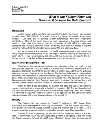
Robotics Math 16-811Sandra MauDecember 2005What is the Kalman Filter andHow can it be used for Data Fusion?MotivationJust to explain a little about the motivation for this topic, the project I was workingon was called “PROSPECT: Wide Area Prospecting Using Supervised AutonomousRobots.” Our goal was to develop a semi-autonomous mutli-robot supervisionarchitecture. One of the major issues for rover navigation is knowing attitude andposition. Our initial idea was to use a combination of IMU, GPS and odometry(encoders and visual) to solve this issue. So for my math project, I wanted to exploreusing the Kalman Filter for attitude tracking using IMU and odometry data.As an additional follow up note, our NASA sponsored project was one of themany projects cancelled following NASA’s change in vision to focusing on methods for alunar return. Thus I unfortunately did not spend too much time developing this KFfurther, though hopefully it will become applicable in some future project.Overview of the Kalman FilterThe Kalman filter can be summed up as an optimal recursive computation of theleast-squares algorithm. It is a subset of a Bayes Filter where the assumptions of aGaussian distribution and that the current state is linearly dependant on the previousstate are imposed. In other words, the Kalman filter is essentially a set of mathematicalequations that implement a predictor-corrector type estimator that is optimal in thesense that it minimizes the estimated error covariance when the condition of a linearGaussian system is met. If the Gaussian assumption is relaxed, the Kalman filter is stillthe best (minimum error variance) filter out of the class of linear unbiased filters. [8]From the time it was developed, the Kalman has been the subject of extensiveresearch and application, especially in the field of navigation. [4] The simple and robustnature of this recursive algorithm has made it particularly appealing. Also, even thoughit is rare that the optimal conditions exist in real-life applications, the filter often worksquite well in spite of this and thus contributes to its appeal. [4]HistoryThe Kalman filter was created by Rudolf E. Kalman in 1960, though PeterSwerling actually developed a similar algorithm earlier. The first papers describing itwere papers by Swerling (1958), Kalman (1960) and Kalman and Bucy (1961). [1] Itwas developed as a recursive solution to the discrete-data linear filtering problem.Stanley Schmidt is generally credited with the first implementation of a Kalmanfilter. In 1959 when NASA was to exploring the problem of navigating to the moon withthe Apollo program, Schmidt at NASA Ames Research Center saw the potential of

extending the linear Kalman filter to solve the problem of trajectory estimation. Theresult was called the Kalman-Schmidt filter (now commonly known as the ExtendedKalman Filter.) By 1961, Schmidt and John White had demonstrated that this filter,combined with optical measurements of the stars and data about the motion of thespacecraft, could provide the accuracy needed for a successful insertion into orbitaround the Moon. The Kalman-Schmidt filter was embedded in the Apollo navigationcomputer and ultimately into all air navigation systems, and laid the foundation forAmes' future leadership in flight and air traffic research. [6]Discrete Kalman Filter AlgorithmThis section describes the filter in its original formulation (Kalman 1960) wherethe measurements are measured and state estimated at discrete points in time. Themathematical derivation will not be given here but can be looked up in variousreferences [4][8]Dynamic systems (this is, systems which vary with time) are often represented ina state-space model. State-space is a mathematical representation of a physicalsystem as a set of inputs, outputs and state variables related linearly. The Kalman filteraddresses the general problem of trying to estimate the state of a discrete-timecontrolled process that is governed by the models below [5]:In addition to this, a random, Gaussian, white noise source wk and vk are addedto the state and observation equations respectively. The process noise w has acovariance matrix Q and the measurement noise v has a covariance matrix R, whichcharacterizes the uncertainties in the states and correlations within it.At each time step, the algorithm propagates both a state estimate xk and anestimate for the error covariance Pk, also known as a priori estimates. The latterprovides an indication of the uncertainty associated with the current state estimate.These are the predictor equations. The measurement update equations (correctorequations) provide a feedback by incorporating a new measurement value into the apriori estimate to get an improved a posteriori estimate. The equations for this recursivealgorithm are shown below:

The Kalman Gain (K in measurement update equation 1) is derived fromminimizing the a posteriori error covariance [4][5]. What the Kalman Gain tells us is thatas the measurement error covariance R approaches zero, the actual measurement z is“trusted” more and more, while the predicted measurement Hxˆ is trusted less and less.On the other hand, as the a priori estimate error covariance P approaches zero theactual measurement is trusted less and less, while the predicted measurement istrusted more and more.Application to researchApparatusFor my experiments, the main sensor readings came from a Crossbow IMU300CC, 6-DOF inertia measurement unit. The three angular rate sensors are vibratoryMEMS sensors that use the coriolis force for measurements and the three MEMSaccelerometers are silicon devices that use differential capacitance for measurements.This IMU was mounted inside the NASA K-10 rover at the turning center of themachine. All measurements were made by polling the IMU through a RS-232 serialport. A Visual C .NET 2003 program was developed to collect data.

Basic Kalman Filter Without Input to Track Constant Value(use basic KF for yaw rate of stationary rover from IMU measurements)One of the classic basic Kalman Filter examples is to track a constant value withnoisy measurements. So this too was my first step. I developed a basic Kalman Filterfor tracking the constant yaw rate value of a stationary rover. The state model for thiswould be:xˆ k 1 ϕ k 1zˆk 1 ϕ k 1which means that coefficients A 1, B 0, H (or sometimes written as C) 1.Since the rover is stationary, the true raw rate should remain stationary at 0, butas can be seen in the figure below, the IMU gyro measurements are very noisy withbias error of up to /- 2 deg/s (according to the manual). It can be seen that running thedata through the Kalman Filter reduces the inaccuracies of the measurements quitedramatically, but is still not yielding the true heading exactly. Ofcourse, how well ittracks the constant depends a lot on the error covariances Q and R. The values I usedwere Q 0.0282 and R 0.0952 based on research from a paper using a similarCrossbow IMU [2].

Basic Kalman Filter Without Input to Track Yaw Angle(integrated yaw rate)The next step was to integrate the yaw rate values to get heading (yaw angle.)From the yaw equation below, the state space model was developed. Note that B 0since there was no additional information input into the system.Running this KF model on about 50 seconds of data from a stationary rover, it wasfound that the angle drifted off by nearly 2.2 degrees. After doing some research, Ifound that the major errors for these low-cost IMUs are bias and drift [7]. I also foundother research that has tried to address this issue by estimating the bias to be able tocompensate the measured value [3][9]. This lead to the next iteration described next.Two-Tier Kalman for Yaw Angle with Yaw Rate Bias CorrectionThe method I used to estimate a bias value was to implement re-modify the basicKF for tracking a constant such that the a priori state estimate for every iteration wasalways zero. By doing this, it means that the deviation from zero in the estimate of ouryaw rate constant results completely from the measurement and noise model (xhat 0 K * [z - 0] K * z ). Thus, this should give us an idea of how much the measurementis biased.Below is the result of the yaw rate bias KF. Compared to the results of the basicyaw rate constant KF, it was observed that the estimate was better. This is because we

are incorporating other known data into the system (i.e. we know the heading should bezero, so we set our a priori estimate to zero based on that knowledge). This illustrates aform of data fusion.After about 20 iterations, P converged to 0.0023 (see second image below). Thismeans that the error covariance of the a posteriori state estimate (x-xhat)2 was 0.0023

[deg/s]2, thus the bias error in the state estimate was the square root of that, or 0.0479deg/s. This value was then used in the basic KF for yaw angle by subtracting eachmeasurement by this bias. The result was quite promising, giving only about 1 degerror after 50 seconds, which is over 100% improvement from KF without biascorrection as can be seen graphically below.One thing of note is that the bias also drifts as time goes on, so any biasestimation would likely become invalid quickly. [3][10] Since bias has a quadratic effecton position derived from IMU [7], it can become a serious problem. One proposedsolution was to stop the rover regularly to recalibrate the bias [3], another was to prefilter the noisy IMU measurements [10] and a third was to get more data to obtain abetter a priori estimate or measurement (a general solution).IssuesThe KF for yaw with bias correction developed above was applied to the roverturning 360 degrees both CW and CCW. It was found that the tracking was not verygood in this instance at all. For both results, the KF yielded about 160 deg rather thanthe actual 360 deg as can be seen below.

The graph itself looks good at the beginning: a flat line indicating when the roverwas still stationary, then a nearly linear slope indicating when the rover was turning at anearly constant velocity. However, I noticed that there is no flat line at the endindicating when the rover stopped turning and became stationary again. This leads meto suspect that it might be that there is a significant communication delay between thetime the IMU is polled for data and when the data is actually read by my code.Another problem might be that the data is not being fast enough for a greatestimate. Right now, the data is being received at 10 Hz. This may be increased bychanging the IMU from polled to continuous mode.

Sensor FusionKalman with Motion Control Input and IMU Measurement to Track Yaw AngleAs was briefly touched upon before, data or sensor fusion can be made throughthe KF by using various sources of data for both the state estimate and measurementupdate equations. By using these independent sources, the KF should be able to trackthe value better. The next iteration for my KF would be to incorporate the wheelvelocities in making the state measurement as seen in the model below.I unfortunately did not have the foresight to collect motor control informationwhich can be converted to wheel velocities to run my code for the above model. I willleave this as future work.ConclusionThe Kalman Filter is the most widely used filter for good reason. It is a verysimple and intuitive concept with good computational efficiency. However, that beingsaid, to implement it just right is somewhat of an art and very dependent on the systemat hand.There are also many variants for Kalman (and more generally, Bayesian) filterswith their respective benefits and drawbacks. It is no wonder that the field is so wellexplored and yet still being developed further.