WIXLIB

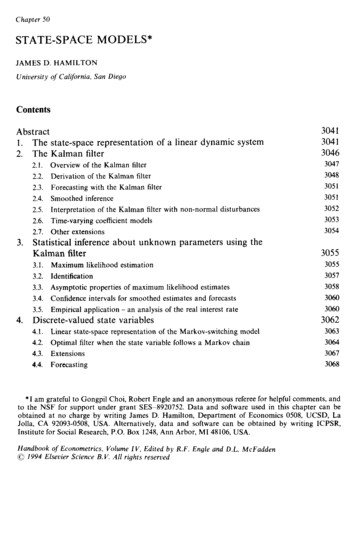
Chapter 50STATE-SPACEJAMESMODELS*D. HAMILTONUniversity of California, San DiegoContentsAbstract1. The state-space representation2. The Kalman filter3.4.2.1.Overview2.2.Derivationof the Kalman2.3.Forecasting2.4.Smoothedof a linear dynamicsystem3047filterof the Kalman3048filterwith the .Time-varying2.7.Otherof the Kalmancoefficientfilter with Statistical inferenceKalman filteraboutunknownparametersusing timation3057of maximumfor smoothed- an analysislikelihoodestimates3058estimates3060and forecastsof the real interest3060rate3062state variablesstate-spacerepresentationof the 74.4.Forecasting3068filter when the state variablefollows a Markovmodel30634.1.chain3064*I am grateful to Gongpil Choi, Robert Engle and an anonymousreferee for helpful comments, andto the NSF for support under grant SES8920752.Data and software used in this chapter can beobtained at no charge by writing James D. Hamilton,Departmentof Economics 0508, UCSD, LaJolla, CA 92093-0508, USA. Alternatively,data and software can be obtained by writing ICPSR,Institute for Social Research, P.O. Box 1248, Ann Arbor, MI 48106, USA.Handbook of Econometrics, Volume 1 V, Edited by R.F. Engle and D.L. McFadden0 1994 Elsevier Science B.V. All rights reserved

J.D. pertiesapplicationof maximum- anotherand rences3069grid oodestimateslook at the real intereststate-space3071modelsfor nonlinear,non-normalfilterto e-spacemodels30773077

3041Ch. 50: State-Space ModelsAbstractThis chapter reviews the usefulness of the Kalman filter for parameter estimationand inference about unobserved variables in linear dynamic systems. Applicationsinclude exact maximum likelihood estimationof regressions with ARMA disturbances, time-varyingparameters, missing observations,forming an inference aboutand specificationof business cyclethe public’s expectationsabout inflation,dynamics. The chapter also reviews models of changes in regime and develops theparallel between such models and linear state-space models. The chapter concludeswith a brief discussion of alternative approachesto nonlinearfiltering.1.The state-spacerepresentationof a linear dynamic systemMany dynamic models can usefully be written in what is known as a state-spaceform. The value of writing a model in this form can be appreciated by consideringa first-order autoregression(1.1)Y, 1 Yr st r,with E, N i.i.d. N(0, a’). Future values of y for this process depend on (Y,, y, 1,. . . )only through the current value y,. This makes it extremely simple to analyze thedynamics of the process, make forecasts or evaluate the likelihood function. Forexample, equation (1.1) is easy to solve by recursive substitution,Yf m 4”y, 4m-1Ey l 4m-2Et 2 . q5l - from which the optimal E form-period-aheadE(Y, ,lY,,Y,-,,.) mY,.(1.2)m 1,2,.,forecastis seen to be(1.3)The process is stable if 14 1 1.The idea behind a state-space representationof a more complicated linear systemis to capture the dynamics of an observed (n x 1) vector Y, in terms of a possiblyunobserved (I x 1) vector 4, known as the state vector for the system. The dynamicsof the state vector are taken to be a vector generalizationof (1.1):5, r F& n, ,.(1.4)

J.D. Hamilton3042Here F denotes an (r x I) matrix and the (r x 1) vector II, is taken to be i.i.d. N(0, Q).Result (1.2) generalizes to5t m F”& F”- I, Fr -rwhere F” denotes v, ,the matrix Fm-2 t 2 .form 1,2,.,F multiplied(1.5)by itself m times. HenceFuture values of the state vector depend on ({,, 4, 1,. . .) only through the currentvalue 5,. The system is stable provided that the eigenvalues of F all lie inside theunit circle.The observed variables are presumed to be related to the state vector throughthe observation equation of the system,y, A’.q H’{, w,.(1.6)Here yt is an (n x 1) vector of variables that are observed at date t, H’ is an (n x r)matrix of coefficients, and W, is an (n x 1) vector that could be described asmeasurementerror; W, is assumed to be i.i.d. N(O,R) and independentof g1 and(1.6) also includes x,, a (k x 1) vector of observedv, for t 1,2,. . Equationvariables that are exogenous or predeterminedand which enter (1.6) through the(n x k) matrix of coefficients A’. There is a choice as to whether a variable is definedto be in the state vector 5, or in the exogenous vector xt, and there are advantagesif all dynamic variables are included in the state vector so that x, is deterministic.However, many of the results below are also valid for nondeterministicx,, as longas n, contains no informationabout & , or w, , for m 0, 1,2,. . . beyond thatyr. For example, X, could include lagged values of y orcontainediny, ,,y, ,,.,variables that are independentof 4, and W, for all T.The state equation(1.4) and observationequation(1.6) constitutea linearstate-space repesentation for the dynamic behavior of y. The framework can befurther generalizedto allow for time-varyingcoefficient matrices, non-normaldisturbancesand nonlineardynamics, as will be discussed later in this chapter.For now, however, we just focus on a system characterizedby (1.4) and (1.6).Note that when x, is deterministic,the state vector 4, summarizes everything inthe past that is relevant for determiningfuture values of y,E(Yt ml51,5r-l,.,Yt,Y1-1,.) EC(A’x, , H’5, , w, ,)l5,,5,-,,.,y,,y,-l,.I A’xy , H’E(5, ,151,&-1,., t, *-l,.) A'x HlF"'&.(1.7)

3043Ch. 50: State-Space ModelsAs a simple example of a system that can be writtena pth-order autoregressionin state-space- 11) 4l(Y, - 4 #dYte 1 - PL) . 4p(Yt-p l(Y, 1- 11) form, consider(1.8)Et 12i.i.d. N(0, a2).E, -Note that (1.8) can equivalentlyas41 42 . 4p-1 4pYt 1 -P1i !Yz - PJ&p 2be written -P10Ol.OO.o0.00Yt - PYc-1 -P.1:011J&p 1:-PEt 10.!I:1 .(1.9)0The first row of (1.9) simply reproduces (1.8) and other rows assert the identityY, j-p Yy, j-pforj O,l,.,p - 2. Equation(1.9) is of the form of (1.4) withr pand& (yt-PL,Yt-1v 2 1-(1.10)-P .#-p l-P)I (1.11)-(% 1,0,.,O)I,F 0.1.0-0The observationYt P (1.12). .‘.equationisH’t,,where H’ is the first row of the (p x ,p) identitybe shown to satisfy(1.13)matrix.The eigenvaluesof F can(1.14)thus stability of a pth-order autoregressionrequires that any value 1 satisfying(1.14) lies inside the unit circle.Let us now ask what kind of dynamic system would be described if H’ in (1.13)

J.D. Hamilton3044is replacedwith a generaly, /J Cl81 0,(1 x p) vector,“. ,-IK(1.15)where the 8’s represent arbitrary coefficients. Suppose that 4, continuesin the manner specified for the state vector of an AR(p) process. Lettingthe jth element of &, this would mean4151,t 142I! 1r 2,t 1r’ PJ 1 .4,-l4%10.000.1.0000.10 1to evolvetjt denoteE t 10.(1.16).0:IThe jth row of this system for j 2,3,. . . , p states that j,l 1 (j- l,f, implyingfor5jt Lj51,t lj 1,2(1.17),., p,for L the lag operator. The first row of (1.16) thus implies that the first elementof 4, can be viewed as an AR(p) process driven by the innovationssequence {E,}:(1.18)(1- l - 2 2- - p P)S1.1 l , l.Equationsy, p (l(1.15) and (1.17) then imply(1.19) B,L’ e2L2 . ep-1LP-1)51r.If we subtractp from both sides of (1.19) and(1 - c ,L- q5,L2 - . - 4,Lp), the result is(1 -&L-4,L2-operateon bothsideswith. - pLP)(yt-p) (l 1L1 2L2 ‘ ep-1LP-1)x (1 - ,L-f#),L2 - . - f#),LP)&, (1 8,L’ 82L2 8p ,LP-1)E,(1.20)by virtue of(1.18). Thusequations(l.15)and(1.16)constitutea state-space representation for an ARMA(p,p - 1) process.The state-space framework can also be used in its own right as a parsimonioustime-series description of an observed vector of variables. The usefulness of forecastsemerging from this approach has been demonstratedby Harvey and Todd (1983),Aoki (1987), and Harvey (1989).

Ch. 50: State-Space Models3045The state-spaceform is particularlyconvenientfor thinkingabout sums ofstochastic processes or the consequencesof measurementerror. For example,suppose we postulate the existence of an underlying “true” variable, &, that followsan AR(l) process(1.21)with u, white noise. Suppose that 4, is not observed directly. Instead, the econometrician has available data y, that differ from 5, by measurementerror w,:Y, 5, wt.(1.22)If the measurementerror is white noise that is uncorrelatedwith t , then (1.21)and (1.22) can immediatelybe viewed as the state equationand observationequation of a state-space system, with I n 1. Fama and Gibbons (1982) usedjust such a model to describe the ex ante real interest rate (the nominal interestrate i, minus the expected inflation rate 7 ;). The ex ante real rate is presumed tofollow an AR( 1) process, but is unobserved by the econometricianbecause people’sexpectation7 : is unobserved.The state vector for this applicationis then , i, - rcr - /J where p is the average ex ante real interest rate. The observed expost real rate (y, i, - n,) differs from the ex ante real rate by the error peoplemake in forecasting inflation,i, - x, p (i, - 7rcp- p) (7 ;- 71J,which is an observation equation of the form of (1.6) with R 1 and w, ( 1 - 7 ).If people do not make systematic errors in forecasting inflation, then w, mightreasonablybe assumed to be white noise.In many.economicmodels, the public’s expectations of the future have importantconsequences.These expectations are not observed directly, but if they are formedrationally there are certain implicationsfor the time-series behavior of observedseries. Thus the rational-expectationshypothesis lends itself quite naturallyto astate-space representation;sample applicationsinclude Wall (1980), Burmeisterand Wall (1982), Watson (1989), and Imrohoroglu(1993).In another interesting econometricapplicationof a state-space representation,Stock and Watson (1991) postulatedthat the common dynamic behavior of an(n x 1) vector of macroeconomicvariables yt could be explained in terms of anunobserved scalar ct, which is viewed as the state of the business cycle. In addition,each series y, is presumed to have an idiosyncraticcomponent(denoted a,J thatis unrelated to movements in yjt for i #j. If each of the componentprocesses couldbe described by an AR(l) process, then the [(n 1) x l] state vector would be4 L a113Qtv . . . 2 a,,)(1.23)

J.D. Hamilton3046with state equationC,al, I1:P2.c,al* :Iyz.IO.l.P”1 1% 00Y “t(1.24)v2,t lequationYl,Y2t1:azr [ j [j{ZGJand observationUC,, 1v1,t 1.0. 1a,,1(1.25)a:ImThus yi is a parameter measuring the sensitivity of the ith series to the businesscycle. To allow for @h-order dynamics, Stock and Watson replaced c, and ai, in(1.23) with the (1 xp) vectors (c,,c, t ,., c,-,, r) and ( ,,,a , , ,., r)sothat 4, is an [(n 1) x l] vector. The scalars C#I in (1.24) are then replaced by(p x p) matrices Fi with the structure of (1.12), and blocks of zeros are added inbetween the columns of H’ in the observationequation (1.25). A related theoreticalmodel was explored by Sargent (1989).State-space models have seen many other applicationsin economics. For partialsurveys see Engle and Watson (1987), Harvey (1987), and Aoki (1987).2.The Kalman filterFor convenience, the general form of a constant-parameteris reproducedhere as equations (2.1) and (2.2).linear state-spacemodelState equation51 1 (r x 1)J-5,Yt(n xequation.4’x, 1)E(w,w;)(r x 1)Q(r x 4E(v, J Observation(2.1) v, 1(r x r)(r x 1)(n x k)(k x 1) R .(n x n) WC&(n x r)(r x 1) w,(n x 1)(2.2)