Transcription
Arbitrage-Free Pricing of XVA for AmericanOptions in Discrete TimebyTingwen ZhouA ThesisSubmitted to the Facultyof theWORCESTER POLYTECHNIC INSTITUTEIn partial fulfillment of the requirements for theDegree of Master of ScienceinFinancial MathematicsMay 2017ADVISORS:Professor Stephan SturmProfessor Gu Wang
AbstractTotal valuation adjustment (XVA) is a new technique which takes multiple material financialfactors into consideration when pricing derivatives. This paper explores how funding costs andcounterparty credit risk affect pricing the American option based on no-arbitrage analysis. Wereview previous studies of European option pricing with different funding costs. The conclusionshelp to compute the no-arbitrage price of the American option in the model with different borrowing and lending rates. Another model with counterparty credit risk is set up, and this pricingapproach is referred to as credit valuation adjustment (CVA). A defaultable bond issued by thecounterparty is used to hedge the loss from the option’s default. We incorporate these two modelsto assess the XVA of an American option. The collateral, which protects the option investors fromdefault, is considered in our benchmark model. To illustrate our results, numerical experiments aredesigned to demonstrate the relationship between XVA and parameters, which include the fundingrates, bond’s rate of return, and number of periods.
Contents1Introduction1.1 Important Terms and Concepts . . . . . . . . . . . . . . . . . . . . . . . . . . . .2European Option2.1 Important theorems of European option . . . . . . . . . . . . . . . .2.2 A comparison between super-hedging price and hedging price . . . .2.3 XVA of European options with funding spread in a one-period model .2.4 XVA of European options with collateral in a one-period model . . . .5. 5. 6. 12. 14XVA of American Options with Funding Spread3.1 Base model of American option pricing . . . . . . .3.2 One-period model with funding spread . . . . . . . .3.3 American option with funding spread in rational case3.4 Multi-period model with funding spread . . . . . . .3.1217171929324XVA of American Options with Funding spread and Counterparty Credit Risk364.1 Credit valuation adjustment for American options . . . . . . . . . . . . . . . . . . 364.2 Multi-period XVA of American options . . . . . . . . . . . . . . . . . . . . . . . 415XVA of American Options with Collateral6Numerical Analysis536.1 XVA of American options without collateral . . . . . . . . . . . . . . . . . . . . . 536.2 XVA of American options with collateral . . . . . . . . . . . . . . . . . . . . . . 557Conclusion4458i
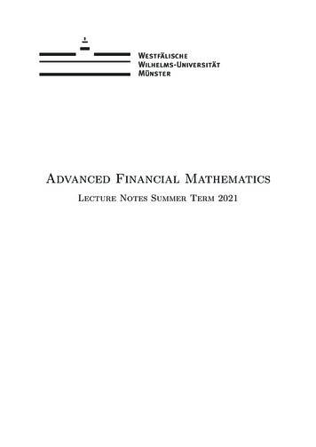
List of Figures3.13.2The American option pricing process in the base model. . . . . . . . . . . . . . . . 18One-period American option pricing process with funding spread from tn to tn 1inside the multi-period model with funding spread. . . . . . . . . . . . . . . . . . 324.1The American option pricing process in the model with counterparty credit riskwhen N 1. . . . . . . . . . . . . . . . . . . . . . . . . . . . . . . . . . . . . . . 405.1The American option transaction process with considering counter-party credit riskand funding spread. This model is incorporated with a collateral account with N 1. 46The American option transaction process with considering counter-party credit riskand funding spread. This model is incorporated with a collateral account in a longposition. . . . . . . . . . . . . . . . . . . . . . . . . . . . . . . . . . . . . . . . . 485.26.16.26.36.4XVA of the American put option when varying the borrowing and lending rates ina 5-period binomial tree model. Other constant parameters are u 1.2, d 0.8,S0 100, K 100, α 0.5, rm 0.25, and h g 1/5. . . . . . . . . . . . . . .XVA of the American put option when varying the number of periods and bond’srate of return. The constant parameters in this two model are u 1.2, d 0.8,S0 100, K 100, α 0.5, rl 0.1, rb 0.2, and h g 1/5. In the left figure,bond’s rate of return is rm 0.25, and the number of periods range from 1 to 10.The right figure is under a 5-period binomial tree model with the bond’s rate ofreturn ranging from 0.1 to 0.4. . . . . . . . . . . . . . . . . . . . . . . . . . . . .XVA of the American put option when varying the borrowing and lending ratesin a 5-period binomial tree model with collateral. Other constant parameters areu 1.2, d 0.8, S0 100, K 100, α 0.5, h g 1/5, γ 0.6, and rc 0.05.XVA of the American put option in the model with collateral when varying thenumber of periods and the bond’s rate of return. The constant parameters in thistwo model are u 1.2, d 0.8, S0 100, K 100, α 0.5, rl 0.1, rb 0.2,h g 1/5, γ 0.6, and rc 0.05. In the left figure, bond’s rate of return isrm 0.25, and the number of periods range from 1 to 10. The right figure is undera 5-period binomial tree model with the bond’s rate of return ranging from 0.1 to 0.4.ii54545556
6.5XVA of the American put option in a 5-period model with collateral when varyingthe collateralization rate from 0.3 to 0.9. Other constant factors are u 1.2, d 0.8, S0 100, K 100, α 0.5, rl 0.1, rb 0.2, h g 1/5, rm 0.25, andrc 0.05. . . . . . . . . . . . . . . . . . . . . . . . . . . . . . . . . . . . . . . . 57iii
List of SymbolsStVt (·)rbrlrcudqq̃ t tMtM tXtXt X t X tΦ(Xt )EtAtγPtstock price at time tthe payoff of option at time tborrowing ratelending ratecollateral ratestock price up factorstock price down factorprobability of counterparty defaultrisk neutral measure of counterparty defaultshares of stock in a long position hedging portfolio at time tshares of stock in a short position hedging portfolio at time tshares of money market account (MMA) in a long position hedging portfolioat time tshares of MMA in a short position hedging portfolio at time thedging portfolio for a long position in a option at time tsuper-hedging portfolio for a long position in a option at time thedging portfolio for a short position in a option at time tsuper-hedging portfolio for a long position in a option at time tvalue of the portfolio X at time tEuropean option price at time tAmerican option price at time tcollateralization rateno-arbitrage price of a portfolio consisted of option and collateral at time tiv
Chapter 1IntroductionIn the past, the traditional approaches which were adopted to price options involve several assumptions. These assumptions deny the difference between the borrowing and lending rates, orany default in the counterparty. Here, the new approach, which relaxes those assumptions whenpricing options, is known as ‘XVA’. It is short for value adjustment for some risk elements, whichis denoted as ‘X’.The difference between borrowing and lending rates is referred to as funding spread. In thispaper, we emphasize the aspects of funding spread and default of the counterparty. By comparingXVA with the traditional approaches, this new approach is more practical and realistic.Both XVA and traditional approaches are pricing the American option under the assumptionthat no arbitrage opportunity exists in the market. In discrete time settings, these two methodsadopt the backward induction approach in the multi-period binomial tree model [4]. The pricingprocess begins at the maturity date, and goes backward to the initial date by calculating the pricestep by step.The paper is organized as follows. In the first Chapter, we introduce some backgrounds ofthe project information and provide the definition of each important term. We review and analyzesome conclusions of the European option price from previous studies in Chapter 2. Some of thefindings are adopted to explore the American option pricing in Chapter 3. The result reveals thatdifferent market conditions will determine the utilization of a hedging portfolio or a super-hedgingportfolio at each time.Chapters 3 - 5 discuss the no-arbitrage price of an American option. The model without fundingspread and default is introduced at first. A funding spread will be added to the model next. Startingwith the one-period model, we extend this to a multi-period model using the backward inductionmethod. The second step focuses on the counterparty credit risk. Defaultable bond is introduced toreplicate the payoff in this situation. After considering funding spread and credit risk separately, weincorporate these two models to compute the XVA. We divide the time interval into two differentkinds of periods. Funding spread and counterparty credit risk are considered separately in these two1
periods. The first period allows the stock and MMA to be traded in the market. Only the defaultablebond is traded in market at the second period. To improve the applicability of the model, we addthe collateral in the model we just constructed. The no-arbitrage price of an American option canbe derived by the value of the portfolio consisting of option and collateral. In Chapter 6, numericalanalyses are offered to demonstrate the relationship between XVA and parameters, which includethe funding rates, bond’s rate of return, and number of periods.1.1Important Terms and Concepts European option: European options are widely traded on exchanges. It can only be exercised on the maturity or expiration date T . On that day, the call option holder can buy, andthe put option holder can sell the underlying asset at a specific price - the exercise price orstrike price.Bonner and Campanelli compute the no-arbitrage European option price by considering theexistence of funding spread and counterparty credit risk in discrete time settings [3]. Incontinuous time settings, Davis, Panas, and Zariphopoulou use the Black-Scholes modelto price the European option [5]. This method considers that there is a transaction costwhen selling and purchasing stocks. Bichuch, Capponi, and Sturm develop the frameworkto compute XVA accounting for funding spread, collateralization, and counterparty creditrisk [2]. Generally, European option’s price is easier to derive than an American option, butsome conclusions from European options can also be applied to price American options. American option: Most of the options traded in the market are American options. Differentfrom the European option, an America option may be exercised before or at the expirationdate. The option buyer needs to optimally choose the time to exercise the option. On theother hand, the seller has the obligation to deliver the exercise payoff to the buyer when theoption is exercised.Multiple approaches have been adopted to value American options. Amin and Bodurthadevelop a discrete time model focusing on risks from currency, domestic term structure, andforeign term structure [1]. Rogers uses the Monte-Carlo simulation to price the Americanoption with simulating the paths of the option payoff [11]. These approaches fail to considerthe risk of default from counterparty and funding spread. Hedging: Hedging is a strategy used to reduce a particular risk faced by the investor. Aperfect hedge is the one that completely eliminates the risk [8]. For example, using futurecontracts is an effective way to hedge the risk from the fluctuation of a product’s price. Sincea perfect hedge can mitigate all of the risks, in this circumstance, the price of the derivativescan be calculated by evaluating the price of the hedging portfolio.The hedging portfolio will generate the same payoff as the derivative. The value of thehedging portfolio is referred to as the hedging price. We use the stock and the money marketaccount (MMA) to construct the hedging portfolios. When we consider the default riskfrom the counterparty, defaultable bonds are also involved in the hedging portfolio. Given2
different borrowing and lending rates, the hedging portfolio’s value may not represent thederivative’s value properly, therefore the super-hedging portfolio would be considered as analternative. Super-hedging: When the market completeness breaks down, which means that the riskcannot be completely eliminated, super-hedging becomes a good way to measure the valueof derivatives. This is a strategy that can at least hedge the risk of the derivative with thelowest cost. The portfolio which is constructed by the strategy of super-hedging is calledthe super-hedging portfolio. It can produce no less than the payoff as the derivative with thelowest price. The value of the super-hedging portfolio is referred to as the super-hedgingprice.The super-hedging portfolio is built with the same components as the hedging portfolio.Even though the super-hedging portfolio will have a better payoff at the maturity, it maynot be as expensive as the hedging portfolio. Their relationship depends on different marketconditions. A comparison of hedging portfolios and super-hedging portfolios will be madein Section 2.3. Collateral: “In lending agreements, collateral is a possession pledged as security for repayment of a loan to a lender, to be forfeited in the event of a default” [7]. This means that ifthe borrower fails to pay the principal and interest based on the lending agreements, the itemacting as collateral can be forfeited to offset the loan.In Chapter 4, we introduce a pricing model with collateral. To eliminate parts of the risk fromthe counterparty’s default, the hedger requires the counterparty to post cash as collateral witha collateralization rate γ. This means if the value of the derivative is C, then the amount ofthe cash collateral is γC. If default do not occur, the collateral receiver will give the collateralprovider rc γC in each period before the maturity date as an interest. rc is called the collateralrate. At the maturity date or the time when the option is exercised, the collateral providerwill receive the full amount of γC. Once the counterparty defaults on the option, this processwill be terminated. The receiver will keep the cash collateral to eliminate the loss from thedefault. Arbitrage: An arbitrage is an investment strategy that yields with positive probability apositive profit and is not exposed to any downside risk [6]. For a portfolio X with initialvalue 0, Φ(Xt ) is the portfolio value at time t. It is an arbitrage strategy if it satisfies thefollowing conditions at a time t up to the maturity date T :1. P(Φ(Xt ) 0) 1.2. P(Φ(Xt ) 0) 0.To compute the XVA of a derivative, we assume that the funding rates are unique to eachhedger. Usually, personal interest is influenced by various factors, such as credit score andeconomic performance [10]. It indicates that the cost of constructing a portfolio is different.Thus, unlike classical option pricing, arbitrage strategies are no longer universal but specificto a hedger. In that way, the XVA of a derivative we derive is unique to each hedger in the3
market.When we discuss the price of the American option in Chapter 3, the price will be affectedby the buyer’s exercising strategy. In Section 3.2, we modify the explanation of arbitrage onthe basis of the definition we have mentioned above. More details will be provided.4
Chapter 2European OptionMany conclusions from European option pricing will be useful to understand no-arbitrage pricingfor American options. In this chapter, we will introduce some important theorems on Europeanoptions pricing from previous research. We will make a comparison between the hedging price andthe super-hedging price given by different market conditions at Section 2.2. On the basis, we willcompute the XVA for a European option with funding spread in a one-period model. In Section2.4, a new model with a collateral account is generated to price European options by consideringfunding spread.2.1Important theorems of European optionThis project is based on the no-arbitrage analysis in the binomial tree model. When the marketconsists of only the stock and the MMA, the no-arbitrage condition can be derived [3]. This can beseen in Theorem 1 below. We have an underlying asset (stock), the price of which at time t is St ,t 0, 1, 2 . . . T . Time zero is the initial time, and time T is the maturity date. We assume that thereis no dividend paid in this model. Any shares of stock and MMA are allowed in the transaction.Also, there is no transaction cost. Then at time t 1, the stock price has two movements, ‘H’and‘T’, the values of which are uSt or dSt respectively. We call u and d the annualized up and downfactors of the stock price with u d. Receptively, rl and rb are the annualized lending rate andborrowing rate.Theorem 1 No-Arbitrage Condition: In a market with stocks and MMAs, under the oneperiod binomial model with the length of h, there is no arbitrage in the market if and only ifu d, d 1 rb , rl rb , and 1 rl u.Adapted from: Bonner and Campanelli [3]Since the borrowing rates and the lending rates are not the same for each individual in the5
market, the no-arbitrage condition is also unique for hedgers. This coincides with what we havementioned in the definition of ‘Arbitrage’.In a discrete time setting, the no-arbitrage price of a European option in one period model,Et , can be derived as the following Theorem 2. As noted in Section 1.1, the price of Europeanoptions are related to the values of the hedging and super-hedging portfolios. Both the hedgingand super-hedging portfolio consist of the underlying asset and MMA. They are constructed givenby the payoffs of the European option. The difference is that hedging portfolio replicates exactlythe same payoff, and the super-hedging portfolio produces at least the same payoff.We denote the portfolio at time t as Xt . Both of these two portfolios have the length of oneyear. It replicates the cash flows of the option from the time period (t,t 1). The superscript ‘*’is used to distinguish whether the portfolio is super-replicating or not. Both the hedging portfolioand super-hedging portfolio are constructed by stocks and MMAs. The subscript ‘ ’ means theportfolio ‘X’ is used in the short position.Theorem 2 Under the assumption of non-zero funding spread, in the one-period binomial treemodel, the no-arbitrage price of the European option at time t satisfies the following condition.More than that, any prices out of this interval can construct arbitrages. ), Φ(X )} E min{Φ(X ), Φ(X )}max{ Φ(X t tttt ), Φ(X )} Φ(X ), then the interval is open on the left:Notes: If max{ Φ(X t t t ). If min{Φ(X ), Φ(X )} Φ(X ), then the interval is open on the right side:Et Φ(X ttttEt Φ(Xt ).Adapted from: Bonner and Campanelli [3]2.2A comparison between super-hedging price and hedgingpriceUnder the no-arbitrage conditions in Theorem 1, we get the price of the European option in Theorem 2. We noticed that both sides of the inequality are decided by comparing the super-hedgingprice and the hedging price. So in this part, we use the no-arbitrage conditions to compare them.For each node at time t, we build a one-period binomial tree model with time length h. Thenthe maturity date T t h. Since the pricing process is backward in a one-period model, we knowthe option value at time t h. We can build the hedging and super-hedging portfolio based onfuture cash flows.6
For the replication portfolio, it involves shares of stock and M shares of MMA. If M 0,then the investor lends money to others, then r takes the value rl . On the other hand, if M 0, theinvestor borrows money, then r takes the value rb . Thus we can write r as:r rl 1M 0 rb 1M 0 .In the following theorems, the proof of those in the short position shares the same approach asthe long position. So we only provide the proof for the latter. For simplification, is short for t ,and M is short for Mt .Theorem 3 In the one-period model with length h at time t, If d 1 rl 1 rb u, Φ(Xt ) ) Φ(X ). This means the super-hedging price is larger than or equal toΦ(Xt ) and Φ(X t tthe hedging price at any time t.Proof: Firstly, we will compute the hedging price and the super-hedging price separately.Without loss of generality, we assume the time length of the one-period model is h 1.The functions used to compute hedging price are as follows: Φ(Xt ) St M,Vt 1 (H) uSt M(1 r), Vt 1 (T ) dSt M(1 r).The functions used to compute super-hedging price are as follows: Φ(Xt ) St M ,Vt 1 (H) uSt M (1 r ), Vt 1 (T ) dSt M (1 r ).Four sub-situations can be derived based on whether the hedger is borrowing or lending moneyin this two portfolios.1. M 0 and M 0In this case, hedger will lend money in the hedging portfolio and super-hedging portfolio.Then r and r take the lending rate, r r rl . Thus, we rewrite the previous functions.Hedging functions: Φ(Xt ) St MVt 1 (H) uSt M(1 rl ) Vt 1 (T ) dSt M(1 rl )7
Super-hedging functions: Φ(Xt ) St MVt 1 (H) uSt M (1 rl ) Vt 1 (T ) dSt M (1 rl )In the hedging functions, we can plug Φ(Xt ) into the right hand side of Vt 1 (H) and Vt 1 (T ).(Vt 1 (H) uΦ(Xt ) (1 rl u)MVt 1 (T ) dΦ(Xt ) (1 rl d)MIn the same way, we rewrite the super-hedging functions. By comparing those functions, wederive two inequalities as follows:(u(Φ(Xt ) Φ(Xt )) (1 rl u)(M M),(2.1)d(Φ(Xt ) Φ(Xt )) (1 rl d)(M M).We first suppose M M in the above inequalities. For the first inequality, since u 1 rl ,we have (1 rl u)(M M) 0, thus Φ(Xt ) Φ(Xt ). On the other direction, we assumeM M. For the second inequality, since d 1 rl , we have (1 rl u)(M M) 0, thusΦ(Xt ) Φ(Xt ). In either cases, we can get the conclusion that the hedging price is less thanor equal to the super-hedging price.2. M 0 and M 0In this case, the hedging portfolio has a negative position in MMAs, and the super-hedgingportfolio has a non-negative position in MMAs. So, we have r rb , and r rl . We rewritethe functions as follows.Hedging functions: Φ(Xt ) St MVt 1 (H) uSt M(1 rb ) Vt 1 (T ) dSt M(1 rb )Super-hedging functions: Φ(Xt ) St MVt 1 (H) uSt M (1 rl ) Vt 1 (T ) dSt M (1 rl )In the hedging functions, we plug Φ(Xt ) into the right hand side of Vt 1 (H) and Vt 1 (T ).(Vt 1 (H) uΦ(Xt ) (1 rb u)MVt 1 (T ) dΦ(Xt ) (1 rb d)M8
In the same way, we rewrite the super-hedging functions. Next, we derive the formula asfollows:(u(Φ(Xt ) Φ(Xt )) (1 rl u)M (1 rb u)M,(2.2)d(Φ(Xt ) Φ(Xt )) (1 rl d)M (1 rb d)M.Since rl rb , the inequalities (2.2) can be transformed to (2.1). Since M 0 M, we haveΦ(Xt ) Φ(Xt ), i.e., the hedging price is less than the super-hedging price.3. M 0 and M 0Following the process in the case M 0 and M 0, we can draw the same conclusion.4. M 0 and M 0Following the process in the case M 0 and M 0, we can draw the same conclusion.In conclusion, under the assumption of d 1 rl 1 rb u, the super-hedging price islarger than the hedging price in a long position. This is also true for a short position.Definition 2.2.1 We say a portfolio is optimal if we cannot rebalance it with a better payoff at anytime after that. A portfolio is not optimal if we can rebalance it with a better payoff at any timeafter that.A nonoptimal portfolio cannot be used as a super-hedging portfolio. A super-hedging portfoliois a portfolio which can produce at least the same payoff as the derivative does with the lowestcost. Since a nonoptimal portfolio can be rebalanced with a better payoff, we can build anotherportfolio which has the same payoff but less expensive. This can be a fraction of the rebalancedportfolio. Then a nonoptimal portfolio is not a super-hedging portfolio. On the other hand, eitherin a long position or a short position, if a hedging portfolio is nonoptimal, it is more expensive thanthe super-hedging portfolio.Theorem 4 If u 1 rb , portfolios consisted of a negative position in MMA are not optimal.Proof: Suppose there are two portfolios. For portfolio A, it has shares of stock and M sharesof MMA, where M 0. For portfolio B, it only has MSt shares of stock. Thus the initial valuesof A and B are the same.For portfolio A, we have M 0, so the funding rate takes the borrowing rate. We can draw atable to show the payoffs of the portfolios in different situations.9
updownAB uSt M(1 rb ) uSt Mu dSt M(1 rb ) dSt MdIn either case, as d u 1 rb , the payoff of portfolio B is better than portfolio A. Thus whenu 1 rb , portfolios consisted of a negative position in MMA are not optimal.Under the condition of u 1 rb , it is not optimal to borrow money. When borrowing money,it means to use the money borrowed to invest in the stock. But the maximum return of the stockis less than the borrowing rate, which means that it will make a loss when borrowing money. Soit is better to invest less in the stock market without borrowing money. The same conclusion goesfor the case when 1 rl d. In this situation, lending money is not optimal. Since the lendingrate will be less than the minimum return of the stock. So using this money to invest in the stockmarket is a better choice. We will prove it in a mathematical way.Theorem 5 If 1 rl d, portfolios consisted of a positive position in MMA are not optimal.Proof: Suppose there are two portfolios. For portfolio A, it has shares of stock and M sharesof MMA, where M 0. For portfolio B, it only has MSt shares of stock. Thus the initial valuesof A and B are the same.For portfolio A, since M 0, it means r rl . We can draw a table to show the payoff of theportfolio at different situations.updownAB uSt M(1 rl ) uSt Mu dSt M(1 rl ) dSt MdIn either case, as 1 rl d u, the payoff of the portfolio B is better than the portfolio A.Thus when 1 rl d, portfolios consisted of a positive position in MMA are not optimal.Combining the conditions of 1 rl d, u 1 rb , and d u, we can get 1 rl d u 1 rb . At this situation, either borrowing and lending money is not optimal. So, we can draw theconclusion of the following theorem.Theorem 6 If 1 rl d u 1 rb , portfolios consisted of MMA are not optimal.10
When holding MMA is not optimal, and a nonoptimal portfolio is not a super-hedging portfolio,we conclude that the super-hedging portfolio will only consist of stocks. Based on that, we canmake a comparison between the hedging price and the super-hedging price when 1 rl d u 1 rb . ) Φ(X ), which meansTheorem 7 If 1 rl d u 1 rb , Φ(Xt ) Φ(Xt ) and Φ(X t tthe super-hedging price is less than or equal to the hedging price at any time.Proof: In the condition of 1 rl d u 1 rb , super-hedging portfolio will not consist ofMMAs. Thus M 0 in the super-hedging portfolio.For the hedging portfolio of a long position, we can generate the following functions. Φ(Xt ) St MVt 1 (H) uSt M(1 r) uΦ(Xt ) (1 r u)M Vt 1 (T ) dSt M(1 r) dΦ(Xt ) (1 r d)MBy solving those functions, the hedging price is computed as follows: Φ(Xt ) St M,t 1 (T ) Vt 1 (H) V,S(u d)t uV(T) dV(H)t 1t 1 M .(u d)(1 r)For the super-hedging portfolio of the long position, we can draw the following functions. Φ(Xt ) StVt 1 (H) uSt Vt 1 (T ) dStAccording to the definition of super-hedging portfolio, Φ(Xt ) max{ Vt 1u(H) , Vt 1d(T ) }.Next, we make the comparison between the hedging price and the super-hedging price.1. uVt 1 (T ) dVt 1 (H) 0In this case, the hedging portfolio takes a positive position in MMA, thus r takes the lendingrate. For the super-hedging portfolio, since Vt 1u(H) Vt 1d(T ) , we have Φ(Xt ) Vt 1d(T ) . Thevalue of the hedging portfolio is as follows:Φ(Xt ) Vt 1 (H) Vt 1 (T ) uVt 1 (T ) dVt 1 (H) ,u d(u d)(1 rl )11
(1 rl d)[dVt 1 (H) uVt 1 (T )] 0.d(1 rl )(u d)Then, we have Φ(Xt ) Φ(Xt ), i.e, the super-hedging price is less than the hedging price.Φ(Xt ) Φ(Xt ) 2. uVt 1 (T ) dVt 1 (H) 0In this case, the hedging portfolio takes a negative position in MMAs, thus r takes the borrowing rate. For the super-hedging portfolio, since Vt 1u(H) Vt 1d(T ) , we have Φ(Xt ) Vt 1 (H). The value of the hedging portfolio is as follows:uΦ(Xt ) Vt 1 (H) Vt 1 (T ) uVt 1 (T ) dVt 1 (H) ,u d(u d)(1 rb )(1 rb u)[dVt 1 (H) uVt 1 (T )] 0.u(1 rb )(u d)Then, we have Φ(Xt ) Φ(Xt ), i.e, the super-hedging price is less than the hedging price.Φ(Xt ) Φ(Xt ) 3. uVt 1 (T ) dVt 1 (H) 0In this case, the hedging portfolio has M 0. Both of the super-hedging portfolio and thehedging portfolio do not have MMA. They share the same value.Thus, taking a long position in the derivative, the super-hedging price is less than or equal tothe hedging price. This is also true for the short position.2.3XVA of European options with funding spread in a oneperiod modelAs is shown in Theorem 2, under the no-arbitrage condition, we have found that the XVA of aEuropean option with funding spread is: max{ Φ(X t), Φ(X t )} Et min{Φ(Xt ), Φ(Xt )}.While, on the left hand side, when it takes the value of the super-hedging price, it is open on theleft hand side. When it takes the value of the super-hedging price in the right hand side, it is openon the right hand side.The no-arbitrage condition in the market with the stock and the MMA is d 1 rb , and 1 rl u. It can generate four sub-situations, which is d 1 rl 1 rb u, 1 rl d u 1 rb ,d 1 rl u 1 rb , and 1 rl d 1 rb u. Under each of these situations, the optionprice can be simplified as follows:1. d 1 rl 1 rb uBased on Theorem 3, the hedging price is less than the super-hedging price for any positionin the Europ
rowing and lending rates. Another model with counterparty credit risk is set up, and this pricing approach is referred to as credit valuation adjustment (CVA). A defaultable bond issued by the counterparty is used to hedge the loss from the option's default. We incorporate these two models to assess the XVA of an American option.