WIXLIB

Thus he is able to get a free lunch which stands as an alternative expression for anarbitrage opportunity. The main assumption is:Financial markets are free of arbitrage.The whole pricing of financial securities rely on this basic assumption and this is justifiedin efficient and transparent markets where no barriers on trading exist. If an arbitrageoccurs, for example due to miss-pricing of a financial security, the efficient price-buildingin markets would cancel this miss-pricing in very short time.Based on this no-arbitrage principle several conclusions can be drawn which are of greatimportance for pricing derivatives.Theorem 1.2.1 (Replication Principle). We consider a financial market with dividendfree assets. If two self-financing trading strategies with value processes V and W coincideat a time point T they coincide at each time point t [0, T ] in between. HenceV (T ) W (T ) V (t) W (t) for all 0 t T.Note that the replication principle is no mathematical theorem, since we have not established a mathematical model so far and cannot state mathematical claims. But wecan give arguments why the replication-principle can be deduced from the no-arbitrageprinciple.Proof. We would like to show that the initial prices V (0) and W (0) of both strategiescoincide and assume first that V (0) W (0).But then we can- initially sell V buy W ,- follow the trade of W and trade opposite to V in (0, T ),- take the payoff W (T ) of W at the end to neutralise the obligation of V (T ) at theend.This strategy would provide an arbitrage opportunity, the risk-less profit V (0) W (0)from the beginning.In the case W (0) V (0) the same arguments work the other way round.1.2.1 Put-Call ParityAs application of the replication principle we will show that there is a correspondencebetween put and call price of an underlying with the same maturity and strike. This isthe so called put-call parity.Theorem 1.2.2 (Put-Call Parity). We consider a put and a call with same strike Kand maturity T on a dividend-free underlying. Let S0 , c, p denote the inital price of theunderling, call and put. Thenp S0 c KB(0, T ).10(1.1)

Proof. To show the assertion we consider two trading strategies.(i) long in put and long in the underlying,(ii) long in call and K long in a T -Bond.Both strategies get a payoff max{S(T ), K} at T due to(K S(T )) S(T ) max{S(T ), K} (S(T ) K) K.The replication principle implies that their initial prices coincide. But this is the claimedequation (1.1) above.The first strategy above underlines the importance of the put-option in risk management.If you buy a stock you face the risk of a downside stock movement. To cover this riskyou can buy in addition a put with strike K. Then your payoff will exceed at least thestrike K. A put can be seen as an insurance contract protecting against downside stockmovements.1.2.2 Chooser-OptionA further application of the replication principle can be given in order to express theprice of a so called chooser-option by a suitable call and put price.We consider a financial market with- deterministic, constant interest rate r 0. This means that the price of a T bondis given by B(t, T ) e r(T t) ,- an underlying S,- puts and calls of all maturities and strikes.A chooser-option gives its holder the right to choose at T1 T a put or a call withstrike K and maturity T . Let ch(T1 , T, K) , c(S0 , T, K), p(S0 , T1 , Ke r(T T1 ) ) denotethe initial price of the chooser-option, the call with maturity T , strike K and the putwith maturity T1 and strike Ke r(T T1 ) . ThenProposition 1.2.3.ch(T1 , T, K) c(S0 , T, K) p(S0 , T1 , Ke r(T T1 ) )Proof. The holder of a chooser-option will take a call in T1 if its more valuable than thecorresponding put. If we denote by c(S(T1 ), T, K) and p(S(T1 ), T, K) their prices in T1 ,then the chooser-option can be seen as a derivative with payoffC (S(T ) K) 1{c(S(T1 ),T,K) p(S(T1 ),T,K)} (K S(T ) 1{p(S(T1 ),T,K) c(S(T1 ),T,K)} .11

The question is how to replicate this payoff. The key observation is that we can reformulate the choose condition by applying the put-call parity. It holdsc(S(T1 ), T, K) Ke r(T T1 ) p(S(T1 ), T, K) S(T1 )and thereforec(S(T1 ), T, K) p(S(T1 ), T, K) S(T1 ) Ke r(T T1 ) .This leads to the replicating strategy:1. At the beginning:- Take a long position in a call with strike K and maturity T- Take a long position in a put with strike Ke r(T T1 ) and maturity T12. at T1 , if S(T1 ) Ke r(T T1 ) :- exercise the put and receive Ke r(T T1 ) S(T1 )- sell the call and receive c(S(T1 ), K, T )- use the received money to buy a put option with strike K and maturity T .3. at T1 , if S(T1 ) Ke r(T T1 ) : hold the call until T .This strategy is self-financing and provides the payoff of the chooser option at T . Thereplication principle implies the above assertion.12

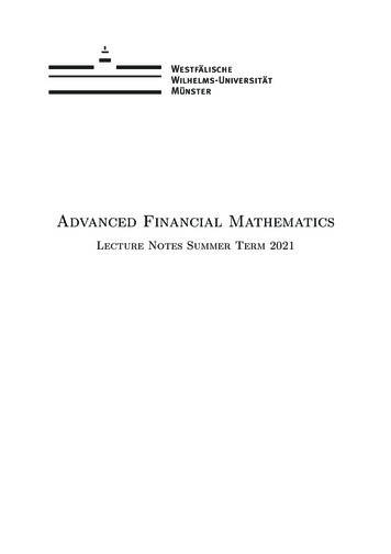
2 The Black-Scholes ModelBlack and Scholes developed in 1971 the approach of pricing derivatives by computingreplicating trading strategies. They were able to derive pricing formulas for plain-vanillaoptions like call and put, in particular the famous Black-Scholes call-price formula. Thebenefits of the model are the following:- simple model- reasonable economic background- analytically tractableThis will be explained in this chapter.2.1 Wiener-ProcessThe Wiener-process, also called Brownian-motion, is one of the most important stochastic processes in continuous time with continuous paths. It is the starting point forthe development of the stochastic integration theory and many sophisticated models inphysics and economics use this process as basic tool. A Wiener-process can be seenas the continuous counterpart of a centered random-Walk and can be constructed aslimiting process of suitable normalised centered random-walks.To be more precise let (Yk )k N be a sequence of identically distributed independentrandom variables with1P(Yk 1) P(Yk 1)2PPutW (1) (t) : tk 1 Yk .By linear interpolation weobtain a continuous time123process with continuous0paths (W (1) (t))t 0 .Enlarge the frequency atfactor n and compress theheight at n Pk1(n) k Define W n j 1 Yj .n13

1n2n3n4n1kn023 Again linear interpolation leads to a continuous time stochastic process W (n) (t) t 0 .This sequence W (n) converges to a limiting process (W (t))t 0 , a Wiener-process.A random-walk is a discrete time stochastic process with independent and stationaryincrements. This property carries over to the limiting process W and can be used togive a precise definition of a Wiener-process.Definition 2.1.1. Let (Ω, F, P) be a probability space and (Ft )t 0 a filtration. Anadapted stochastic-process W (W (t))t 0 is called standard Wiener-process if it fulfills the following properties1. W (0) 0 P-a.s.2. W (t s) W (t) is independent of Ft for all s, t 03. W (t s) W (t) has the same law as W (s) for all s, t 04. W (t) is N(0, t) distributed for all t 05. The paths of W are P-a.s. continuous.Usually we omit the adjective standard and speak of a Wiener-process when a standardWiener-process is meant.Martingales play an essential role in many fields of probability theory, in particular infinance and stochastic analysis.Definition 2.1.2. An adapted process M is called an (Ft )t 0 martingale if the followingholds1. E M (t) for all t 0.2. E(M (t s) Ft ) M (t) for all t, s 0.The independence of the increments can be used to easily identify basic martingaleswhich will play a role in the following.Proposition 2.1.3. Let W be a Wiener-process w.r.t. a filtration (Ft )t 0 . Then thefollowing process are martingales.1. W (t)t 014

2. (W (t)2 t)t 03. (exp(θW (t) 12 θ2 t))t 0 for each θ R.The proof of this assertion is very easy and can be done by carefully exploiting theindependence of increments property. The last martingale is an example of a so calledexponential martingale and can be used to define further probability measures. Thetherefore needed tool is a generalisation of Bayes-Theorem.Theorem 2.1.4 (Change of measure). Let (Ω, F, P) be a probability space with filtration(Ft )t 0 . Let L be a positive martingale w.r.t. P and P̄ a further probability measure on(Ω, F, P) such thatdP̄ F L(t) for all t 0.dP tThen(i) The conditional expectation w.r.t. P̄ can be calculated by computing the conditionalexpectation w.r.t. P. More precisely, if Y is measurable w.r.t. Ft and integrablew.r.t. P̄, then for s tE(Y L(t) Fs )Ē(Y Fs ) .L(s)(ii) M is a P̄-martingale if and only if M L is a P-martingale.(iii) Let R be a positive P-martingale with ER(t) 1 for all t 0. Then a probabilitymeasure QT can be defined on each FT bydQT F R(t) for all t T.dP tProof. (i): We use the definition of conditional expectation directly. For A Fs wegetZZZZE(Y L(t) Fs )E(Y L(t) Fs )dP Y dP̄ Y L(t)dP dP̄.L(s)AAAAThis yields the first assertion.ad (ii): This follows from (i) due to(Mt ) is a P-martingale E(Mt Fs ) Msfor all s t1 E(Mt Lt Fs ) Msfor all s tLs E(Mt Lt Fs ) Ms Lsfor all s t M L is a P-martingale15

ad (iii) Due to ER(T ) 1 an equivalent probability measure on (Ω, FT ) is defined byZR(T )dP for all A FT .QT (A) ADue todQT F E(R(T ) Ft ) R(t)dP tfor all t T the assertion follows.The preceding theorem can be used to state a first simple version of Girsanov’s theoremTheorem 2.1.5 (Girsanov). Let (Ω, F, P) be a probability space with filtration(Ft )t 0and W a Wiener-process w.r.t. P. Let Pϑ be a further probability measure on (Ω, F)such that1dPϑ Ft exp(ϑW (t) θ2 t) L(t) for all t 0.dP2ThenW̄ (t) W (t) ϑt, t 0defines a Wiener-process w.r.t. Pθ .Proof. One has to verify that W̄ satisfies the defining properties of a Wiener-processw.r.t. Pϑ . Clearly W̄ starts at 0 and has continuous paths. To show that the incrementsare independent we consider g : R R measurable and bounded. ThenEϑ (g(W (t) W (s)) Fs ) E(g(W (t) W (s))Lt Fs )1Ls1with Lt exp(ϑW (t) ϑ2 t)2 E(g(W (t) W (s) ϑ(t s))Lt Fs )Ls1 E(g(W (t) W (s) ϑ(t s)) exp(ϑ(W (t) W (s)) ϑ2 (t s)) Fs )21 2 Eg(W (t) W (s) ϑ(t s)) exp(ϑ(W (t) W (s)) ϑ (t s))21 2 Eg(W (t s) ϑ(t s)) exp(ϑW (t s) ϑ (t s))2 Eϑ g(W (t s))Hence, W̄ (t) W̄ (s) is independent of Fs and equally distributed as W̄ (t s) with aN(0, t s)-distribution due to16

1Eϑ g(W (t)) Eg(W (t) ϑt) exp(ϑW (t) ϑ2 t)21 Eg(W (t) ϑt) exp(ϑ(W (t) ϑt) ϑ2 t)2Z1 2 e 2 ϑ t g(x)eϑx N ( ϑt, t)(dx)Z1 211ϑ t2 eg(x)eϑx exp( (x ϑt)2 )dx2tZ2πt1 21 g(x)e 2t x dxZ 2πt g(x)N (0, t)(dx)The Wiener-process W fulfills a further property which is of interest in finance for pricingbarrier options. This is the so called reflection principle.Let τ be a stopping time with P(τ ) 1 . Then the reflected process w.r.t. τ isdefined by(W (t)for t τŴ (t) (2.1)W (τ ) (W (t) W (τ )) for t τThe reflection principle states that Ŵ is also a Wiener-process. This can be proven byexploiting the strong Markov property of the Wiener-process. A useful application isthe computation of the joint distribution of W (T ) and M (T ) supt T W (s).Theorem 2.1.6. Let W denote a Wiener-process and M its running maximum. Thenfor x R and z x it holdsx 2zxP(W (T ) x, M (T ) z) Φ( ) Φ( )TTwith Φ denoting the distribution function of the N(0, 1)-distribution.For the process X defined by X(t) W (t) at it followsx 2z aTx aT ) e2az Φ().P(X(T ) x, sup X(t) z) Φ( t TTTProof. For x R and z x we consider the first time that W reaches z, i.e.τ inf{t 0 : W (t) z}and denote by Ŵ the reflected process w.r.t. τ . Then Ŵ is a Wiener-process andP(W (T ) x, M (T ) z) P(Ŵ (T ) z z x, M (T ) z)17

P(Ŵ (T ) 2z x, sup Ŵ (t) z) P(Ŵ (T ) 2z x)t Tx 2z Φ( )TBut this impliesP(W (T ) x, M (T ) z) P(W (T ) x) P(W (T ) x, M (T ) z)xx 2z Φ( ) Φ( ).TTwhich yields the first formula.To prove the second formula we change the measure by applying Girsanov’s theoremand introducing1dPa Ft exp(aW (t) a2 t) for all t T.dP2Then W has the same distribution w.r.t. Pa as X w.r.t. P. HenceP(X(T ) x, sup X(t) z) Pa (W (T ) x, M (T ) z)t TZ1 exp(aW (T ) a2 T )dP2{W (T ) x,M (T ) z} Eg(W (T ))1{M (T ) z}with g(y) exp(ay 21 a2 T )1( ,x] (y).Due to the first formula the condition distribution function fulfills(1if x zP(W (T ) x M (T ) z) Φ( x ) Φ( x 2z )TTif x z.P(M (T ) z)Taking derivative w.r.t. x yields the conditional densityh(y) 1yy 2z(ϕ( ) ϕ( ))T P(M (T ) z)TTfor all y z. This impliesZ Eg(W (T ))1{M (T ) z} P(M (T ) z)g(y)h(y)dy Z x1yy 2z1 (ϕ( ) ϕ( )) exp(ay a2 T )dy 2TTT x aTx 2z aT Φ( ) e2az Φ(),TTsinceZx 1y1 ϕ( ) exp(ay a2 T )dy2TT18(2.2)

1 E1{W (T ) x} exp(aW (T ) a2 T )2x aT Pa (W (T ) x) Pa (W (T ) aT x aT ) Φ( )Tandx1y 2z1 ϕ( ) exp(ay a2 T )dy2TT 1 E1{W (T ) 2z x} exp(a(W (T ) 2z) a2 T )2 exp(2az)Pa (W (T ) 2z x)x 2z aT exp(2az)Φ()TZ2.2 Pricing in the Black-Scholes ModelThe Black-Scholes model is a continuous time model for a financial market that consistsof- a money market account with price process β(t) ert for all t 0 and- a risky asset with price-process1S(t) S(0)eµt exp(σW (t) σ 2 t).2The process W denotes a Wiener-process and µ, σ, r can be seen as parameters that fixthe distribution.- The number µ R denotes the so called rate of return and affects the expectedevolution of the risky asset, sinceES(t) eµtfor all t 0.- The value σ 0 affects the fluctuation of the risky asset due toVar log(S(t)) Var σW (t) σ 2 tS(0)and is often called volatility.- The interest rate r R represents the evolution of a risk-free money marketaccount.19

To take into account the time-value of money the so called discounted price-process isintroduced byS (t) S(t)1 S(0)e(µ r)t exp(σW (t) σ 2 t) for all t 0.β(t)2We observe that only for µ r the discounted price-process is a martingale. In this casethe risky asset has the same expected return as the money market account and we saythat the market is risk-neutral. The question arises whether starting from µ a change ofthe stand-point, a change of measure, can be done such that the market is risk-neutral.This consideration is incorporated in the term equivalent martingale measure.Definition 2.2.1. We consider a Black-Scholes model along the running-time T . Anequivalent martingale measure P is a probability measure on (Ω, FT ) with the followingproperties1. P and P are equivalent probability measures on (Ω, FT ).2. The discounted price process S (t) S(t)β(t), 0 t T is a martingale w.r.t. P .An application of Girsanov’s theorem provides the existence of an equivalent martingalemeasure.Theorem 2.2.2. In a Black-Scholes model with running-time T 0 an equivalentmartingale measure exists.Proof. We know form 2.1.5 that an equivalent probability measure P can be defined by1dP Ft L(t) exp(ϑW (t) ϑ2 t) for all t T.dP2The parameter ϑ has to be chosen such that the discounted price process becomes amartingale. Since W (t) W (t) ϑt is a Wiener-process w.r.t. P we obtain1S (t) S(0)e(µ r)t exp(σW (t) σ 2 t)21(µ r)t S(0)eexp(σ(W (t) ϑt) σ 2 t)21 2(µ r σϑ)t S(0)eexp(σ(W (t) σ t)2Thus S is a martingale if and only ifµ r σϑ 0 and the theorem is proven.20ϑ µ rσ

The existence of an equivalent martingale measure is an important property of the BlackScholes model. It opens a probabilistic way to pricing derivatives. As we will see laterin the course all financial derivatives with an integrable payoff C at T can be replicatedand the initial value of each replicating strategy coincides with the expected discountedpayoff under the equivalent martingale measure. Therefore the following definition isjustified.Definition 2.2.3. Let P be the equivalent martingale measure in the Black-ScholesC . Then the initialmodel and C be an FT -measurable payoff at T with E β(T)arbitrage-free price of C is defined byp0 (C) E C E C .β(T )Later we will clarify why this definition is reasonable. Simply speaking, pricing of aderivative with payoff C at T means- determine a reasonable equivalent martingale measure P - compute E C This pricing mechanism is reasonable in more or less all financial market models andmainly used in practise.Before we give some applications we note that S is a positive martingale under P . Thusa further equivalent change of measure can be done by defining a probability measureP σ viadP σS (t)1 exp(σW (t) σ 2 (t))Ft dPS(0)2for all t T . Girsanov provides thatW (t) W (t) σtis a Wiener-process w.r.t. P σ .To give a full picture we have the following evolution of the stock price process underthe different measure- The subjective probability measure P:1S(t) S(0)eµt exp(σW (t) σ 2 t)2- The equivalent martingale measure P :1S(t) S(0)ert exp(σW (t) σ 2 t)2- The further transformed measure P σ :S(t) S(0)e(r σ2 )t211exp(σW (t) σ 2 t)2

This means that S is a geometric Wiener-process with- trend µ and volatility σ w.r.t P,- trend r and volatility σ w.r.t. P ,- trend r σ 2 and volatility σ w.r.t. P σ .This can be exploited by deriving the Black-Scholes formula.Theorem 2.2.4. We consider a call with maturity T and strike K in a Black-Scholesmodel with volatility σ and initial stock price S(0). Then the initial arbitrage-free priceof the call is given byc(S(0), T, σ, K) S(0)Φ(h1 (S(0), T ) Ke rT Φ(h2 (S(0), T )(2.3)with S(0)K (r 21 σ 2 )T h1 (S0 , T ) σ Tlog S(0) (r 21 σ 2 )TK h2 (S0 , T ) .σ TlogProof. In the first step we computeE e rT (S(T ) K) E? e rT ST 1{ST K} E? e rT K 1{St K}S? S(0)E? T 1{ST K} e rT KE? 1{ST K}S(0)? S(0) Pσ (ST K) e rT K P? (ST K) {z} {z}(1)(2)To compute the probabilities we remind you on the representation of S under P andP σ . It follows KST? logPσ (ST K) Pσ logS(0)S(0) 1K?22 Pσ σWT σ T (r σ )T logS2S(0) K W ?log S(0) 12 σ 2 T (r σ 2 )T T? Pσ T σT {z } N (0,1) 1 2log S(0) (r σ)TK2 . Φ σ T22

and STKP (ST K) P log logS(0)S(0) 1K?2 P σWT σ T rT log2S(0) K W? 12 σ 2 T rT logS(0) T? P T σT {z}? N (0,1) Φ log S(0)K (r 21 σ 2 )T . σ THence (2.3) follows.Note that due to the put-call parity the price of a put can be easily calculated too. Putand call are examples of so called path independent options since the payoff at maturityis only a function of the terminal stock-price. More delicate is the problem of findingpricing formulas for path dependent options. This can be done for so called one-sidedbarrier options.Theorem 2.2.5. A down and out call with maturity T , strike K and barrier B S(0)is an option with payoff (S(T ) K) at maturity T if the barrier B is not hit duringthe running-time. This corresponds to a derivative with payoffC (S(T ) K) 1{inf t T S(t) B} .The initial price of a down and out call is given byp0 (C) c(S0 , T, K) (S0 2bS2) σ c(S0 , T, K 02 )BB(2.4)with b σr 21 σ .This means that the price of a down and out call can be expressed by call prices w.r.t.different strikes.Proof. Nearly the same calculations as in the ordinary call can b

Financial markets are free of arbitrage. The whole pricing of nancial securities rely on this basic assumption and this is justi ed in e cient and transparent markets where no barriers on trading exist. If an arbitrage occurs, for example due to miss-pricing of a nancial security, the e cient price-building