Transcription
Raster Scanning: A New Approach to Image Sonification,Sound Visualization, Sound Analysis And SynthesisWoon Seung Yeo and Jonathan BergerCCRMA, Department of Music, Stanford Universitywoony@ccrma.stanford.eduAbstractRaster scanning is a technique for generating or recordinga video image by means of a line-by-line sweep, tantamountto a data mapping scheme between one and two dimensionalspaces. While this geometric structure has been widely usedon many data transmission and storage systems as well asmost video displaying and capturing devices, its applicationto audio related research or art is rare.In this paper, a data mapping mechanism of raster scanningis proposed as a framework for both image sonification andsound visualization. This mechanism is simple, and producescompelling results when used for sonifying image texture andvisualizing sound timbre. In addition to its potential as across modal representation, its complementary and analogous property can be applied sequentially to create a chainof sonifications and visualizations using digital filters, thussuggesting a useful creative method of audio processing.Special attention is paid to the rastrogram - raster visualization of sound - as an intuitive visual interface to audio data.In addition to being an efficient means of sound representation that provides meaningful display of significant auditoryfeatures, the rastrogram is applied to the area of sound analysis by visualizing characteristics of loop filters used for aKarplus-Strong model. Construction of new sound synthesissystems based on texture analysis / synthesis of the rastrogram is also discussed.1 IntroductionData conversion between the visual and audio domain hasbeen an active area of scientific research and various multimedia arts. Examples include waveforms, spectrograms, andnumerous audio visualization plug-ins, as well as visual composition and image sonification software such as Metasynth(U&I Software ) and Audiosculpt (IRCAM ).Since these conversions essentially represent data mappings, it is crucial to understand and utilize the nature ofFigure 1: Raster scanning.datasets in both audio and visual domains to design an effective mapping scheme. The temporal nature of a sound andthe time-independent, two-dimensional nature of an imagerequires that data mappings between the two media addressthese fundamental differences.1.1 Raster Scanning as a Data MappingRaster scanning is a technique for generating or recordingthe elements of a display image by sweeping the screen ina line-by-line manner. More specifically, it scans the wholearea, generally from left to right, while progressing from topto bottom of the imaging sensor or the display monitor, asshown in figure 1.In addition to being the core mechanism behind most videodisplay and capturing devices, geometric framework of rasterscanning - a mapping between one- and two-dimensional dataspaces - can be found in other places such as communicationand storage systems of two-dimensional datasets. This is, infact, the property that receives primary attention in our choiceof raster scanning as a new mapping framework between image and sound.Raster scanning provides an intuitive, easy to understandmapping scheme between one- and two-dimensional data spaces.This simple, one-to-one mapping also makes itself a totallyreversible process: data converted into one representation canbe reconstructed without any loss of information.
2 Review of Comparable WorksTogether with almost every introduction of devices whichcould record and store audio and/or visual media information,numerous attempts have been made to convert data from onedomain into the other. Among other works in the early days,special attention is paid to the technique of animated sounddeveloped by McLaren (McLaren and Jordan 1953), in whichhe “drew” lines and curves on the audio portion of his filmsto create the sound for his motion pictures. In spite of beingpossibly subjective and unclear, his method has a huge implication in that, for each picture frame, it was a mapping fromtwo-dimensional stationary images to one-dimensional timedependent sounds.Computer technology and digital media formats openedup a new world for multimedia art, pioneered by Whitney(Whitney 1980) and others. By constructing a highly organized set of data mappings between musical events and visual motion patterns/colors, Whitney combined both domainsto create “an inseparable whole that is much greater than itsparts:” instead of being satisfied with only unidirectional conversions, he had the vision of interchangeability between audio and visual domains, and emphasized the advantage andpower of digital media that enabled it.In terms of geometric framework, applications of rastermapping to sound-image conversions can rarely be found.However, there are some comparable works based on different types of scanning methods.2.1 Sound ScannerIn (Kock 1971), Kock used a “sound scanner” to makesound visible: he put a small microphone to a long motorized arm which swept out a raster-like arc pattern. Attachedto the microphone was a small neon light driven by an amplifier connected to the microphone. Sound received by themicrophone would then light up the lamp, which was photographed in darkness with a long exposure. The resultingpicture, therefore, depicted the sound level as bright patterns.While the result of our raster visualization is time dependent, Kock’s work was spatial rather than temporal; althoughthe light source swept the space over a period of time, itsresults were standing waves. In terms of loudness to brightness conversion, however, they are based on a similar mapping rule.2.2 Spiral Visualization of Phase PortraitTo visualize period-to-period difference of a sound, Chafe(Chafe 1995) projected phase portrait of a sound onto a timespiral, thereby separating each period. In this mapping, timebegins at the perimeter and spirals inward, one orbit corresponding to one full period of the waveform. Also, tracecan be colored according to specific spectral qualities of thesound.Spiral drawing path, together with the use of spectral transform, sets this technique apart from raster visualization. However, it should be noted that this was proposed as an analysistool for designing physical synthesis models, especially withpitch-synchronicity in mind. Application of the raster mapping method to a similar problem will be discussed in §5.2.3 Wave Terrain SynthesisIn wave terrain synthesis (Bischoff, Gold, and Horton 1978),a “wave surface” is scanned in an “orbit” (a closed path),and movement of the orbit causes variations in the generated sound. Obviously this is a mapping from two- to onedimensional data space, which is applicable to image sonification.Techniques that scan a wave terrain have been explored byseveral researchers, including (Borgonovo and Haus 1984).None of them, however, are similar to the raster scanning pathwe propose.2.4 Scanned SynthesisScanned synthesis (Verplank, Mathews, and Shaw 2000)is a sound synthesis technique which “scans” a closed path ina data space periodically to create a sound. Due to its emphasis on the performer’s control of timbre, data to be scanned isusually generated by a slow dynamic system whose frequencies of vibration are below about 15 [Hz], whereas the pitch isdetermined by the speed of the scanning function. The systemis directly manipulated by motions of the performer, thereforecan be looked upon as a dynamic wavetable control.While scanned synthesis can be characterized by variousscanning patterns and data controllability, raster sonificationfeatures a fixed geometric framework dedicated to convertingrectangular images to sound.2.5 Research on Mapping GeometryIn (Yeo 2001), Yeo proposed several new image sonification mappings whose scanning paths and color mappings aredifferent from those of the inverse spectrogram method thatis most widely used. Examples include vertical scanning, andscanning along a virtual “perpendicular” axis, with horizontalpanning.This research for mapping geometry has been further refined in (Yeo and Berger 2005) to provide the concept ofpointer - path pair, which serves as the basis of a generalframework for mapping classification.
2.6 Significance and ContributionsIn summary, the following can be proposed as possiblecontributions of this research in relation to existing works. By adopting raster scanning method, we can construct asimple and reversible mapping framework between image and sound with complementarity. This enables usnot only to utilize images as sound libraries (or soundsas image libraries), but also to edit sounds by modifying corresponding images (or vice versa), in a highlypredictable way.Figure 2: Rules of raster mapping. Raster sonification creates a sound which evokes the visual texture of the original image in detail. Although itlacks the freedom of control provided by scanned synthesis, its geometric framework proves to be highly effective with two-dimensional images. Raster visualization is also proposed as an intuitive toolfor timbre visualization, sound analysis, and filter design for digital waveguide synthesis. Moreover, combination of raster sonification and visualization not only suggests a new concept of soundanalysis and synthesis based on image processing techniques, but also has strong implications for artistic applications, including cross-modal mapping and collaborative paradigm.3 Image SonificationCurrently, raster mapping for sonification is defined asfollows: Brightness values of grayscale image pixels, rangingfrom 0 to 255 (8-bit) or 65535 (16-bit), are linearlyscaled to fit into the range of audio sample values from-1.0 to 1.0. One image pixel corresponds to one audio sample.Figure 2 illustrates these rules.3.1 Basic PropertiesBecause of the natural periodicity found in the majority ofimages, the sonified result of an image sounds “pitched:” thewidth of an image determines the period (thereby the pitch) ofits sonified sound. Also, by the one-to-one sample mapping,area of an image corresponds to the duration of its sonifiedsound.In addition to width, pattern changes in the vertical direction are represented as similar changes in timbre over time.(a) Sawtooth.(b) Sine.(c) Pulse frequency modulation.(d) Pulse width modulationFigure 3: Images with constant and changing vertical patterns. Sonified results are specified individually.This is depicted in figure 3: images in 3(a) and 3(b) sonifies into sounds with constant sound quality, whereas 3(c) and3(d) are exaples of time-varying timbre.3.2 Texture SonificationRaster mapping proves to be highly effective when usedfor sonifying the fine “texture” of an image. Sonified soundspreserve the feeling of the original images quite similarly inthe auditory domain, and are quite useful for discriminatingrelative differences between various image textures. Figure 4illustrates four images with contrasting textures: a number oftests have shown that most people could correctly match theoriginal images with their sonified sounds when they weregiven all of them simultaneously.Providing an absolute auditory reference to a particularvisual texture, however, is a challenging task. To this end,construction of a large set of image-sound pairs as a mappinglibrary, together with their classification and training, is desirable.
(a)(b)display a waveform of a one-second long sound recorded atthe sampling rate of 48 [kHz] without any loss of sample, animage with the width of 48,000 pixels is needed. Same sound,however, can fit into a rastrogram with an area containingthe same number of pixels (i.e., 240 200), viewable withinmost computer display. Naturally, sound duration contributesto the image area (and height).4.1 Width And Pitch Estimation(c)(d)Figure 4: Images used to compare textures by sound.(a) Original.(b) “Patchwork”.(c) “Grain”.Figure 5: Comparison of visually filtered images.3.3 Effects of Visual FiltersRaster mapping also produces interesting and impressiveresults when used for sonifying the effects of various visualfilters. Figure 5 contains an image together with its filteredresults. Sonified results of these images are very convincing.Compared with the sound generated from the original imageof figure 5(a), sound of figure 5(b) produces the auditory image of small bumpy texture, while that of figure 5(c) feelsmore noisy and grainy.Sonification of visual filter effects could be further developed as the concept of “sound manipulation using imageprocessing techniques” when combined with correspondingraster visualization.4 Sound Visualization: RastrogramVisualization of sound with raster mapping is an inverseprocess of raster sonification. Values of an audio samples (from -1.0 to 1.0) are linearly scaled to fit into the range of brightness values ofimage pixels (within the range from 0 to 255). One audio sample corresponds to one image pixel.A new term rastrogram is proposed as its name.Compared with ordinary waveform displays and/or spectrograms, rastrogram can be considered to be highly spaceefficient - equally as much as spectrogram. For example, toRastrogram is basically a representation of short segmentsof audio samples stacked from top to bottom over time. Sinceit shows the phase shift between each of those segments, rastrogram can be a useful tool for visualizing changes of pitchover time.To make this effective, its width should be properly chosen to match the length of one period of sound as closelyas possible, thereby being pitch-synchronous. In case of anexact match, every “stripe” of rastrogram should align ona perfectly vertical direction. Due to the limited precisionof frequency values obtained by integer-only image widths,however, unwanted “drifts” can be introduced by round-offerrors: stripes will usually slope in either way, depending onthe instantaneous pitch value.Figure 6 shows three rastrograms that are generated fromthe same violin sound, but of different width. Obviously 6(b)is most well-synchronized to its pitch, which is supposed tobe around 44, 100/170 259.4[Hz]. From a closer inspection of this, we see the followings: Inclination at a certain point provides the amount ofrelative delay to the width of rastrogram, which makesit possible to derive more precise pitch. Figure 6(b)shows that the original sound could be largely segmentedinto five different pitch sections, with roughly estimatedpitch values of 259.3 [Hz] (I), 259.5 [Hz] (II), 259.4[Hz] (III), 259.2 [Hz] (IV), and 259.6 [Hz] (V), respectively. In addition, it is clearly shown that there are a numberof short, subtle changes of pitch throughout the duration of sound. These include the relatively big one inthe beginning of the sound (O), which introduces temporary pitch shift down to about 257.9 [Hz].It should be noted that rastrogram visualizes fine detailsof pitch variations with extremely high precision in both timeand frequency, which can hardly be achieved by spectrogramalone.
(a) fm 1[Hz].(b) fm 2[Hz].(c) fm 5[Hz].(d) fm 10[Hz].(e) fm 20[Hz].(f) fm 50[Hz].Figure 7: Rastrograms of frequency modulated sounds,y(t) cos [2π{fct I ·fm ·sin(2πfm t)}], with fc 220.5[Hz], I 1, but different f m values (as specified).4.2 Frequency Modulation(a) 171 pixels.(b) 170 pixels.(c) 169 pixels.Figure 6: Comparison of rastrograms from the same violinsound, but of different widths (as specified). Sound samplewas obtained from the Musical Instrument Samples of Electronic Music Studios, University of Iowa.Rastrograms of frequency-modulated sounds with different values of modulation frequency are depicted in figure 7.With the same modulation index, threshold of image “clarity”lies around 10[Hz] of modulation frequency, which roughlymatches the perceptual characteristics in the auditory domain.Figure 8 shows the results of various modulation indices.Compared with the previous case of modulation frequency,image patterns remain relatively clear for higher values ofmodulation index.Rastrograms of FM sounds with higher modulation frequency and index values are generally complex, and requirefurther research to be analyzed and fully understood. On thecontrary, sounds with relatively low modulation frequencyand moderate modulation index produce quite simple rastrograms, from which both parameters could be derived. Also,they show a wood-like texture.This, in turn, means that selected woodgrain images asin figure 9(a) could be raster sonified to synthesize FM-likesounds. Figure 9(b) shows a simplified “synthetic” rastrogram, which is generated from an FM synthesizer whose parameters were designed to emulate this natural woodgrain.Except for the fine details of the natural woodgrain side, soundsof both figures are quite similar to each other in terms of pitch.
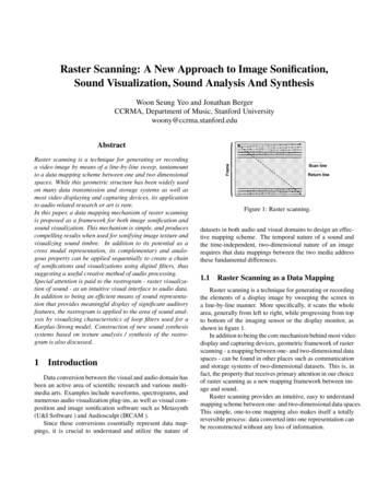
(a) Original.(b) PFiltered by y[n]91k 0 x[n k].10 (c) With noise.Figure 10: Rastrograms of sounds modified by different audioprocesses.(a) I 2.(b) I 5.(c) I 10.Figure 11: System diagram of Karplus-Strong algorithm,with a simple loop filter.4.3 Effects of Audio Filters(d) I 20.(e) I 30.(f) I 40.Figure 8: Rastrograms of FM sounds from the same equationas in figure 7 . Each sound is generated with f c 220.5 [Hz]and fm 1 [Hz], but with different I (as specified). Notethat I 1 would be the same as figure 7(a)We suggest the idea of “visualizing the effect of audiofilters” as a dual to its counterpart in the other domain. Infigure 10, sound generated from 10(a) is lowpass-filtered andvisualized back to create the rastrogram in 10(b), while 10(c)is converted from the same sound of 10(a) with added whitenoise.Naturally, this could develop further into the idea of “image manipulation with audio filters, which will be discussedin §7.5 Visualization of Karplus-Strong Model(a) Natural woodgrain image.(b) “Synthetic” woodgrain createdfrom an FM sound with fc 220.5[Hz], fm 0.7[Hz], and I 0.6.Figure 9: Woodgrain images.As mentioned in 4.1, rastrogram shows short segmentsof audio samples in order of time. For digital waveguidesound synthesis models, it becomes a visual record of delayline status at every cycle and depicts particular characteristics of the system. This, therefore, becomes an ideal methodto visualize sounds generated from Karplus-Strong algorithm(Karplus and Strong 1983) (Jaffe and Smith 1983), whose diagram with a simple (or, possibly the simplest) filter is shownin figure 11.Figure 12 illustrates rastrograms generated from a KarplusStrong model using different filters in the feedback path. Inthis comparison, inclined lines in each rastrogram receive primary attention. Inclination in the rastrogram of a waveguide represents an additional delay whose length can be determined by degree, thereby showing instantaneous pitch change,as discussed in §4.1. The loop filters used here can be considered as fractional delays using linear interpolation: delay
6 Image Processing Techniques forSound SynthesisWhen used together, raster sonfication and visualizationmake it possible to modify/synthesize a sound using variousimage processing techniques.6.1 Basic Editing and Filtering(a) 0.9 0.1z 1 .(b) 0.5 0.5z 1 .(c) 0.1 0.9z 1 .Figure 12: Rastrograms of plucked-string sounds generated from Karplus-Strong algorithm, with different loop filterH(z)s as individually specified. Delay line length N is 337,which corresponds to about 130.9 [Hz].From the aforementioned geometric properties of rastermapping, it is obvious that time scale modification and frequency shifting of a sound can be performed by resizing itsrastrogram. More precise control of frequency would be possible by parallelogram-shaped skew transforms to considerthe roundoff drift. Other geometric modifications, such asrotation, can change the timbre and pitch: as a special case,rotation by 180 produces a time-reversed sound.In addition to these processes, visual filters can be appliednot only to replace corresponding audio filters but also to create unique variations of the original sound, as suggested byexamples in §3.3.6.2 Texture Analysis and Synthesis(a) 0.05 0.9z 1 (b)0.05z 2 .13 13 z 1 13 z 2 .(c) 0.45 0.1z 1 0.45z 2 .Figure 13: Rastrograms of the same Karplus-Strong model asfigure 4.1, with different second-order loop filter H(z)s thatintroduce one sample delay.sizes of the filters used in 12(a), 12(b), and 12(c) are 0.1, 0.5,and 0.9, respectively. From inspection of figure 12, we seethat each of these coincides the inclination of correspondingrastrogram expressed as x/ y.In Figure 13, Karplus-Strong rastrograms with secondorder loop filters are depicted. Each of these can be considered as a second-order interpolation that is equivalent to onesample delay, thereby having the same degree of inclination.Differences between their amplitude response characteristics,however, are clearly visualized: obviously, the result of 13(a)is not much affected, while 13(c) is the most lowpass-filtered.From the results presented in this section, we can see thatrastrogram produces an effective visualization of particularfeatures of the loop filter used in Karplus-Strong algorithm,including the length of interpolated delay. Although rastrogram does not provide any precise measurement of filter parameters by itself, it has a strong potential as a visual interfaceof a filter analysis/design tool.Numerous algorithms for analysis and synthesis of visualtexture have been developed in the filed of computer graphics, as summarized in (Wei 1999). We believe that these techniques can be used for analyzing the rastrogram of a soundto create a new synthesized one, which then can be rastersonified to produce a visually synthesized version of the original sound. Advantages of using texture synthesis techniquesfor sound include the followings: While preserving the quality of the original image, synthesized textures can be made of any size, providingfull control over the pitch and duration of raster sonified sound. Texture synthesis can also produce tileable images byproperly handling the boundary conditions: this enables us to eliminate any unwanted noise componentsintroduced by abrupt jumps at the edge. Potential applications of image texture synthesis includede-noising, occlusion fill-in, and compression. Therefore, techniques for these could be applied to similarproblems in audio domain.Future research on this topic will be focused on constructing a set of visual eigenfunctions which can span various rastrograms with “auditory significance”. We believe this willprovide a simpler and more effective algorithm for analysisand resynthesis of complex tones.
6.3 Hybrid Synthesis ModelA carefully designed image analysis algorithm might beable to divide a rastrogram into multiple sections dependingon the existence of particular visual patterns. This, with a setof proper mappings between image patterns and sound synthesis algorithms, leads to the idea of hybrid sound synthesisalgorithm: a sound could be created as a series of multiplesegments, each of which is generated from a specific synthesis method chosen by the visual pattern of equivalent imagesection.7 Chained Audio/Visual ConversionsIn §4.3, we have seen the use of raster sonification andvisualization for converting the effect of audio filters. This,when combined with the ideas in §6, constitutes a frameworkof chained conversions between audio and visual domains:audio and visual processes can be connected to each otherthrough raster sonification and visualization, thereby forminga long chain of cross modal conversions.It should be noted that the reversible, one-to-one natureof raster mappings makes these conversions more than a random transformation: data converted into the other domainstill contains its original “meaning”, not only artistically butalso mathematically.Also, to fully understand how filters in one domain affectsignals in the other, relationship between one and two dimensional signal processing techniques is to be investigated. Thehelical coordinate system (Claerbout 1998) would serve as aframework which enables us to analyze two-dimensional datawith methods for one-dimensional space.8 Online ExamplesExamples presented in this paper, together with soundfiles, are available at (Yeo 2006).9 ConclusionWe have here proposed raster scanning method as a newmapping framework for image sonification and sound visualization. Raster sonification proves to be a powerful methodfor creating a sound which contains the “feeling” of the original image, and becomes the elementary background for sonifying the effects of visual filters. Rastrogram, on the otherhand, has a strong potential as a visual interface to audio:in addition to being a space-efficient audio data display, itcan intuitively visualize the timbre and some fundamentalauditory properties of a sound, and filter characteristics aswell. Together, both sides of raster mappings form a completecircle of conversion between audio and visual data, therebymaking it possible to utilize image processing methods forsound analysis and synthesis.Future works will also include artistic applications of rastermappings. In addition to the simple idea of using images assound libraries, sonification of a painting will be proposed asan auditory clue for its visual patterns. Also, the chain ofaudio-visual conversion will be developed into a new framework of collaborative art.ReferencesBischoff, J., R. Gold, and J. Horton (1978). Music for an interactive network of microcomputers. Computer Music Journal 2(3), 24–29.Borgonovo, A. and G. Haus (1984). Musical sound synthesis bymeans of two-variable functions: Experimental criteria andresults. In Proceedings of the International Computer MusicConference, pp. 35–42. ICMA.Chafe, C. (1995, September). Adding vortex noise to wind instrument physical models. In Proceedings of the InternationalComputer Music Conference, pp. 57–60. ICMA.Claerbout, J. (1998). Multidimensional recursive filters via a helix. Geophysics 63, 1532–1541.IRCAM. Audiosculpt. http://forumnet.ircam.fr/ .Jaffe, D. A. and J. O. Smith (1983). Extensions of the karplusstrong plucked string algorithm. Computer Music Journal 7(2), 56–69.Karplus, K. and A. Strong (1983). Digital synthesis of pluckedstring and drum timbres. Computer Music Journal 7(2), 43–45.Kock, W. (1971). Seeing Sound. New York: Wiley-Interscience.McLaren, N. and W. Jordan (1953, Spring). Notes on animatedsound. The Quarterly of Film, Radio, and Television 7(3),223–229.U&I Software. Metasynth 4. http://uisoftware.com/MetaSynth/ .Verplank, B., M. Mathews, and R. Shaw (2000, September).Scanned synthesis. In Proceedings of the International Computer Music Conference. ICMA.Wei, L. (1999). Deterministic texture analysis and synthesis using tree structure vector quantization. In Proceedings of TheSIGGRAPH. ACM.Whitney, J. (1980). Digital Harmony : on The Complimentarityof Music and Visual Art. Peterborough, NH: McGraw Hill.Yeo, W. S. (2001). Image sonification: Image to sound.http://www.mat.ucsb.edu/ (2006).Rasterscanning.http://ccrma.stanford.edu/ woony/works/raster/ .Yeo, W. S. and J. Berger (2005, September). Application of imagesonification methods to music. In Proceedings of The Internaional Computer Music Conference. ICMA.
Figure 1: Raster scanning. datasets in both audio and visual domains to design an effec-tive mapping scheme. The temporal nature of a sound and the time-independent, two-dimensional nature of an image requires that data mappings between the two media address these fundamentaldifferences. 1.1 Raster Scanning as a Data Mapping