Transcription
JOINT TRANSPORTATIONRESEARCH PROGRAMINDIANA DEPARTMENT OF TRANSPORTATIONAND PURDUE UNIVERSITYPile Driving Analysis for Pile Designand Quality AssuranceRodrigo Salgado, Vibhav Bisht, Monica PrezziSPR-3407 Report Number: FHWA/IN/JTRP-2017/15 DOI: 10.5703/1288284316514
RECOMMENDED CITATIONSalgado, R., Bisht, V., & Prezzi, M. (2017). Pile driving analysis for pile design and quality assurance (Joint Transportation Research Program Publication No. FHWA/IN/JTRP-2017/15). West Lafayette, IN: Purdue University. https://doi.org /10.5703/1288284316514AUTHORSRodrigo Salgado, PhDCharles Pankow Professor in Civil EngineeringLyles School of Civil EngineeringPurdue University(765) 494-5030salgado@purdue.eduCorresponding AuthorVibhav BishtGraduate Research AssistantLyles School of Civil EngineeringPurdue UniversityMonica Prezzi, PhDProfessor of Civil EngineeringLyles School of Civil EngineeringPurdue University(765) 494-5034mprezzi@purdue.eduCorresponding AuthorACKNOWLEDGMENTSThe assistance of JTRP staff and, in particular, the support received from INDOT technical staff and the Study Advisory Committee members is much appreciated. The authors are also thankful for the continuous support receivedfrom the project administrator, Mr. Timothy Wells, and the business owner, Mr. Athar Khan, as well as the supportreceived from the SAC members, Mr. Mir Zaheer and Mr. Jose Ortiz.JOINT TRANSPORTATION RESEARCH PROGRAMThe Joint Transportation Research Program serves as a vehicle for INDOT collaboration with higher education institutions and industry in Indiana to facilitate innovation that results in continuous improvement in the planning,design, construction, operation, management and economic efficiency of the Indiana transportation /index htmlPublished reports of the Joint Transportation Research Program are available at http://docs.lib.purdue.edu/jtrp/.NOTICEThe contents of this report reflect the views of the authors, who are responsible for the facts and the accuracy ofthe data presented herein. The contents do not necessarily reflect the official views and policies of the Indiana Department of Transportation or the Federal Highway Administration. The report does not constitute a standard,specification or regulation.COPYRIGHTCopyright 2017 by Purdue University. All rights reservedPrint ISBN: 978-1-62260-479-1
1. Report No.2. Government Accession No.TECHNICAL REPORT STANDARD TITLE PAGE3. Recipient's Catalog No.FHWA/IN/JTRP-2017/154. Title and Subtitle5. Report DatePile Driving Analysis for Pile Design and Quality AssuranceAugust 20176. Performing Organization Code7. Author(s)8. Performing Organization Report No.Rodrigo Salgado, Vibhav Bisht, Monica PrezziFHWA/IN/JTRP-2017/159. Performing Organization Name and Address10. Work Unit No.Joint Transportation Research ProgramPurdue University550 Stadium Mall DriveWest Lafayette, IN 47907-205111. Contract or Grant No.SPR-340713. Type of Report and Period Covered12. Sponsoring Agency Name and AddressIndiana Department of TransportationState Office Building100 North Senate AvenueIndianapolis, IN 46204Final Report14. Sponsoring Agency Code15. Supplementary NotesPrepared in cooperation with the Indiana Department of Transportation and Federal Highway Administration.16. AbstractDriven piles are commonly used in foundation engineering. The most accurate measurement of pile capacity is achieved frommeasurements made during static load tests. Static load tests, however, may be too expensive for certain projects. In these cases,indirect estimates of the pile capacity can be made through dynamic measurements. These estimates can be performed either throughpile driving formulae or through analytical methods, such as the Case method.Pile driving formulae, which relate the pile set per blow to the capacity of the pile, are frequently used to determine whether the pile hasachieved its design capacity. However, existing formulae have numerous shortcomings. These formulae are based on empiricalobservations and lack scientific validation. This report details the development of more accurate and reliable pile driving formulaedeveloped from advanced one-dimensional FE simulations. These formulae are derived for piles installed in five typical soil profiles: afloating pile in sand, an end‐bearing pile in sand, a floating pile in clay, an end‐bearing pile in clay and a pile crossing a normallyconsolidated clay layer and resting on a dense sand layer. The proposed driving formulae are validated through well-documented casehistories of full-scale instrumented driven piles. The proposed formulae are more accurate and reliable on average than other existingmethods for the case histories considered in this study.This report also discusses the development of a pile driving control system, a fully integrated system developed by Purdue that can beused to collect, process, and analyze data to estimate the capacities of piles using the Case method and the pile driving formulaedeveloped at Purdue.17. Key Words18. Distribution Statementdynamic measurements, pile resistance, pile driving formulae,Case analysisNo restrictions. This document is available to the public through theNational Technical Information Service, Springfield, VA 22161.19. Security Classif. (of this report)UnclassifiedForm DOT F 1700.7 (8-69)20. Security Classif. (of this page)Unclassified21. No. of Pages2522. Price
EXECUTIVE SUMMARYPILE DRIVING ANALYSIS FOR PILE DESIGNAND QUALITY ASSURANCEtransmission of data collected in a PC located at a suitable distance from the driving operation. The PDCS can estimate thecapacity of a single pile using existing dynamic methods, e.g., theCase method, or through the pile driving formulae developed atPurdue University.IntroductionFindingsDynamic measurements are often used to predict the capacity ofa pile in the form of (a) pile driving formulae that relate the pile setper blow to the capacity of the pile or (b) analytical methods suchas the Case method that predict the pile capacity from the accelerations and strains measured at the pile head. However, accurateprediction of pile capacity remains a challenge due to the complexresponse of piles during driving, prevailing uncertainties in theresponse of piles under static loading conditions post driving,and uncertainties stemming from simplifications made in thedevelopment of existing formulae.For this study, a fully integrated pile driving control system(PDCS) prototype was developed that collects, processes, and analyzesdynamic data. To develop pile driving formulae, advanced andrealistic soil models that explicitly consider important parameters,such as soil and pile variability, were used to accurately simulatethe hammer-pile-soil system during driving and to predict thecapacity of piles under static loading conditions after driving.The integrated PDCS collects dynamic data through sensorsand modules during pile driving operations. The system conforms to all requirements specified in the pertinent ASTM standard (ASTM D4945). The PDCS uses wireless signals for theComparisons between the capacities predicted using the piledriving formulae developed at Purdue and existing formulae,including the modified-Gates formula used by INDOT, for severalwell-documented case histories of full-scale instrumented drivenpiles have revealed that the pile driving formulae developed at Purdueperform better on average than other formulae. As a result, anintelligent QA/QC program for piling can use this new tool for asubset of routine piling projects, reserving other approaches forlarger projects.ImplementationThe PDCS has been subject to very limited field testing (development was done in the laboratory). Additional testing is necessaryto determine the robustness and reliability of the first integratedPDCS prototype. An ideal testing scheme would be to test thesystem for a variety of hammer systems, pile types, and soil profilesand to compare the capacities predicted from the PDCS using theCase method and the pile driving formulae to capacities measuredin fully instrumented static load tests.
CONTENTS1. INTRODUCTION . . . . . . . . . .1.1 Background . . . . . . . . . . . . .1.2 Problem Statement Summary1.3 Objectives and Organization .11112. PILE DRIVING FORMULAE . . . . . . . .2.1 Introduction . . . . . . . . . . . . . . . . . . .2.2 Soil Reaction Model . . . . . . . . . . . . . .2.3 Development of Pile Driving Formulae2.4 Case Studies . . . . . . . . . . . . . . . . . . .2.5 Summary and Conclusions . . . . . . . . .11247133. THE PILE DRIVING CONTROL SYSTEM (PDCS) .3.1 Introduction . . . . . . . . . . . . . . . . . . . . . . . . . . . .3.2 Data Acquisition . . . . . . . . . . . . . . . . . . . . . . . . .3.3 Data Analysis . . . . . . . . . . . . . . . . . . . . . . . . . . .3.4 Using the PDCS. . . . . . . . . . . . . . . . . . . . . . . . . .14141516174. SUMMARY AND CONCLUSIONS . . . . . . . . . . . . . . . . . . . . . . . . . . . . . . . . . . . . . . . . . . . . . . . . 20REFERENCES . . . . . . . . . . . . . . . . . . . . . . . . . . . . . . . . . . . . . . . . . . . . . . . . . . . . . . . . . . . . . . . . . 20
LIST OF TABLESTablePageTable 2.1 Traditional pile driving formulas2Table 2.2 Soil parameters for typical soil profiles6Table 2.3 Hammer and pile parameters6Table 2.4 Coefficients of pile driving formulas for closed-ended steel pipe piles7Table 2.5 Coefficients of pile driving formulas for precast concrete piles7Table 2.6 Case studies for closed-ended steel pipe piles in kips9Table 2.7 Case studies for precast concrete piles: measured and estimated loads in kips10Table 2.8 Summary of hammer, pile and soil information used in the pile driving formulas in the case studies10Table 2.9 rQ values for predicted pile capacities with different pile driving formulas13
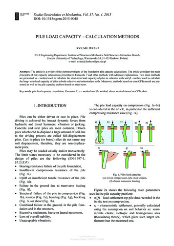
LIST OF FIGURESFigurePageFigure 2.1 Shaft reaction model consisting of three parts: rheological shear band model at the soil-pile interface, a near-field continuumand far-field consistent spring and radiation dashpot3Figure 2.2 Base reaction model consisting of a nonlinear spring and a radiation dashpot attached in parallel3Figure 2.3 Typical pile-soil profile systems found in pile design: (a) piles in sand of uniform density; (b) a floating pile in clay; (c) an endbearing pile in sand; (d) an end-bearing pile in clay; (e) a pile crossing clay resting on sand5Figure 2.4 Comparison between capacity predicted by proposed formulae, calculated static capacity, capacity predicted by Janbu formulaand capacity predicted by PCUBC formula for closed-ended steel pipe piles and concrete piles: (a) piles in sand of uniform density;(b) end-bearing piles in sand; (c) floating piles in clay; (d) end-bearing piles in clay; (e) end-bearing piles crossing clay and resting on sand9Figure 2.5 Bias and variability—as expressed by (a) average rQ and (b) MAPE—for proposed formula, CAPWAP prediction, modified-Gatesformula, modified ENR, Danish formula, PCUBC formula, and Janbu formula14Figure 3.1 Schematic sketching typical arrangement of strain transducers and accelerometers for dynamic testing in: (a) pipe piles (b) H-piles(after ASTM D4945-12 2012)15Figure 3.2 Transducers used in the PDCS: (a) accelerometer (b) strain transducer16Figure 3.3 Main form of PDCS18Figure 3.4 Establishing a wireless connection18Figure 3.5 Observation of blows during the pile driving process19Figure 3.6 Performing Case analysis in the PDCS19Figure 3.7 Entering the Case damping factor in the PDCS19Figure 3.8 Parameters in the pile driving formula form20
1. INTRODUCTION1.1 BackgroundPile resistances must exceed required resistance levels(as dictated by structural loadings); however, if resistances exceed requirements by large margins, projectsresult uneconomical. The most important goal of QA/QCis then to allow contractors to install piles that ownerscan verify to be reliably but not excessively above specified resistances. This can be accomplished through pileload testing.Pile load testing in the field adds to the overall costof projects. Both static and dynamic tests can and aredone with different frequencies on production piles.The costliest but also the most reliable are static pileload tests on instrumented piles. Dynamics tests includeboth pile monitoring during driving (for driven piles)and re-strike tests (tests done some time after pile installation). Although simpler in concept, static load teststend to be reserved for large projects. A less expensivealternative that can offer real-time estimation of pilestatic resistance are dynamic pile load tests, which can beperformed during pile driving (pile driving monitoring)but also at any time after pile installation as re-striketests. Pile monitoring consists of recording the pileacceleration and axial strain at the pile head duringdriving. The pile head velocity histories can be extracted from the recorded acceleration history throughnumerical integration. The recorded strain is used forcalculating the axial force history at the pile head. Thisinformation can be used to deduce the static pile capacity. In pile re-strike tests, the pile head is struck by ahammer after it has been fully driven into the ground.Determination of the pile capacity from static piletests is simple, direct and straightforward. Pile capacityestimation from dynamic tests has always been morechallenging, requiring a dynamic analysis that providesa link between the measurements during pile drivingand the static pile resistance.An accurate, precise relationship between measurements during pile driving and static resistance can provide simplicity and economy to piling projects, allowingengineers to monitor pile driving and indicate to a contractor or inspector that the static resistance requirements have been met before driving of a pile is stopped,avoiding overdriving while at the same time providingconfidence in that the required pile capacities will beavailable. Additionally, reprocessing of the data in theoffice can provide refined estimates of static pile resistance and flag any piles as potentially defective ones.These goals can best be attained through the development of a system that allows the collection, processingand analysis of data.and (2) safety is not compromised (no significant underdriving takes place). The accommodation of theserequisites requires the development of a system that isflexible, meaning that it can be developed further toaccommodate what engineers and researchers learn withadditional work and research on its use, and simple touse, with the implication that engineers will be able touse it without having to face a steep learning curve.1.3 Objectives and OrganizationThe main goal of the research is the development ofthe method and modified analysis, with the prototypesystem being a means to an end. In Chapter 2, wedescribe the methodology for the development of thepile driving formulae and show that they outperformexisting formulae on average in predicting pile capacities from instrumented full-scale static pile load tests.In fact, they perform better than dynamic load testingfor the case histories considered. In Chapter 3, we discussthe configuration and features of the pile driving control system. The operation of the system is explained toprovide guidance to the operator. Chapter 4 provides asummary of the results and conclusion obtained fromthis study.2. PILE DRIVING FORMULAE2.1 IntroductionThe complex interactions between the hammer,cushion, pile and soil, coupled with the significantchanges in the state of the soil around the pile imposedby the driving process, makes the reliable estimationof pile capacity a difficult task. One of the tools usedto assess whether a pile has reached the requiredcapacity are the pile driving formulae. Pile drivingformulae, which relate the pile set per blow to thecapacity of the pile, have been used extensively due totheir simplicity and economic advantages. Approximately 80% of projects in the Indiana Department ofTransportation (INDOT) lack resources for dynamictesting and thus use pile driving formulae (Salgado &Zhang, 2012). Traditionally, pile driving formulae aredeveloped based on energy conservation principles—the energy of the hammer (ram) on impact, after considering energy losses on impact from the variousdriving components between the hammer and the pilehead, is equal to the work done by the total pile resistance for the observed pile displacement after a blow,plus any energy losses on account of dissipation insidethe pile and soil. This can be expressed mathematically as:eh WH H Qult (szsc )1.2 Problem Statement SummaryA significant amount of piling work is carried outby INDOT, necessitating the usage of economicaland reliable methods to ensure that (1) piling is doneeconomically (no significant overdriving takes place)ð2:1Þwhere WH is the hammer (ram) weight; H is thehammer drop height; eh is the hammer efficiency; Qult isthe ultimate pile capacity; s is the observed pile set;and sc is an empirical constant expressing the aforementioned energy losses.Joint Transportation Research Program Technical Report FHWA/IN/JTRP-2017/151
TABLE 2.1Traditional pile driving formulas.FormulaModified-Gates formulaModified ENREquations1Danish formulaeh EhQu szC1rffiffiffiffiffiffiffiffiffiffiffiffiffieh Eh LC1 2AEPacific Coast Uniform Building Code(PCUBC) formula2eh Eh C1szC2WH zkWPC1 WH zWPQu LC2 AEeh E hQu Ku sJanbuNotespffiffiffiffiffiffiQu 1:75 Eh ðlog N{100Þ 11:25eh EhWH zn2 WPQu WH zWP1000 szC 12Qu Eh in ft-lbfC 5 0.1 inn 5 0.5 for steel-on-steel anvil on steel or concrete pilesAll symbols in SI unitsk 5 0.25 for steel piles and 0.1 for all other pilesWPCd �ffi!lKu Cd 1z 1zCdl eh E h LAEs21Units unless explicitly specified: Qu 5 predicted pile capacity (in kips), eh 5 hammer efficiency; Eh 5 maximum driving energy of the hammer(in kip-ft); N 5 number of hammer blows for 1 in. of pile set; s 5 observed pile set in ft; WH 5 weight of the ram (in kips); WP 5 weight of the pile(in kips); L 5 length of the pile (in ft); A 5 cross-sectional area of the pile (in ft2); E 5 Young’s modulus of the pile (in kips/ft2).2The calculation of predicted static capacity using PCUBC formula requires iterations.Equation 2.1 is solved by entering the observed pileset s as input and computing the pile capacity Qult.Several pile driving formulae are based on thisapproach, albeit with varying simplifying assumptionsand empirical adjustments. Available pile driving formulae in the literature, among others, include themodified-Gates formula used by INDOT (2016), themodified ENR (1965) formula, the Danish formula(Olson & Flaate, 1967), the Janbu formula (Bowles,1996) and the Pacific Coast Uniform Building Code(PCUBC) formula (Bowles, 1996). These formulae arelisted in Table 2.1, and will be used for comparisonslater in in this report.Despite being important factors determining responseto driving, existing formulae do not explicitly accountfor the soil type (e.g., sand or clay) surrounding the pileor the pile type (e.g., floating pile or end-bearing pile).Consequently, the predictions from pile driving formulae are often inaccurate and unreliable (McVay,Birgisson, Zhang, Perez, & Putcha, 2000). A critique ofthese formulae can be found in Likins, Fellenius, andHoltz (2012). These shortcomings of pile driving formulaeare accounted for by using factors of safety, recommendations of which may be as large as six (Bowles, 1996).Salgado (2008) notes that large recommended factors ofsafety often diminish the advantages offered by existingformulae in deep foundation quality control. Thus,there exists a need for improved pile driving formulasexhibiting greater reliability and accuracy that wouldconsequently require smaller factors of safety.2In this report, the pile driving process is simulatedusing the soil reaction models developed by Salgado,Loukidis, Abou-Jaoude, and Zhang (2015). Pile drivingformulae are then developed based on the results from aseries of parametric simulations for five general cases:piles in uniform sand deposits, floating piles in clay,end-bearing piles in sand, end-bearing piles in clay andpiles crossing soft clay and bearing on sand. These arevalidated by comparing the results from well-documentedcase histories of static load tests on driven piles and theirperformance is compared with existing formulas listed inTable 2.1. The next section details the soil reaction modeland the methodology used for the development of the piledriving formulae.2.2 Soil Reaction ModelAn advanced soil model was developed by Salgadoet al. (2015) that explicitly took into account soil nonlinearity and hysteresis in order to accurately capturethe complex states of soil during pile driving, and contained input parameters with a physical meaning. Thesemodels were validated by comparing their predictionwith measured pile driving data for two fully instrumented, full-scale pile load tests.The driving process was analyzed using onedimensional analysis. The pile was discretized intosegments, each of which contained a commensurate proportion of the mass of the pile, and was connected to thesegments above and below via linear elastic springs thatJoint Transportation Research Program Technical Report FHWA/IN/JTRP-2017/15
Figure 2.1 Shaft reaction model consisting of three parts: rheological shear band model at the soil-pile interface, a near-fieldcontinuum and far-field consistent spring and radiation dashpot (after Salgado et al., 2015).Figure 2.2 Base reaction model consisting of a nonlinear spring and a radiation dashpot attached in parallel (after Salgadoet al., 2015).model the axial stiffness of the pile. Since the pile helmetsand cushion were not modelled explicitly, the impact ofthe hammer was modelled by an instantaneous application of a velocity corresponding to the energy transferredfrom the hammer to the pile that was calculated byconsidering all energy losses stemming from the impactprocess. The energy losses could be computed from thedynamic measurements during dynamic load tests and,for all practical purposes, are equal to the hammerenergy transfer ratio (ETR). ETR values can take a rangeof values that vary with the type of the hammer and thetype of the pile being driven. According to the Rausche(2000) database, the average ETR values for drop hammers is 0.55, whereas the average ETR for diesel hammers, single acting air/steam hammers, and hydraulichammers varies from 0.25 to 0.8.The reaction model for the soil surrounding theshaft, shown in Figure 2.1, contains three components:(1) a rheological model representing the thin shear bandformed between the interface of the pile and the soil;(2) a continuum soil disk representing the near field soilsurrounding the shaft of the pile; and (3) far-fieldconsistent boundaries placed at the outer boundary ofthe soil disk. The rheological model is adopted fromthe work of Randolph and Simons (1986). It consistsof a viscous dashpot and a plastic slider connected inparallel to each other. Sliding initiates at the pile-soilinterface when the stress ts exceeds the unit limit shaftresistance qsL. Until sliding initiates, the stress in thesoil at the pile-soil interface is equal to the reactionforce experienced by the pile at that segment, afterwhich the viscous dashpot is activated. The viscousdashpot is a power function of the relative velocitybetween the pile and the first node of the near fieldcomponent. The continuum approach (Honeyman, 1985)is used to capture the nonlinear stress-strain relationship of the soil in the near-field. The far field boundariesare used to absorb waves travelling radially away fromthe pile.The soil reaction model at the base of the pile(Figure 2.2) consists of a non-linear spring that considers the non-linear response of the soil under the pilebase and the effect of the loading rate on the baseresistance, and a radiation dashpot that distinguishesbetween the different types of damping. The dashpotand spring are connected to each other in parallel.The non-linear spring follows a hyperbolic load-settlement relationship that is consistent with the responseobserved in static pile load tests. The effect of loadingrates is considered by setting the limit base resistance asa power function of the base. The effects of embedmentdepth and hysteretic damping in the far field are considered by the damping coefficient that was calculated fromFLAC simulations of an embedded oscillating footing.Joint Transportation Research Program Technical Report FHWA/IN/JTRP-2017/153
2.3 Development of Pile Driving FormulaeA series of 1D pile driving simulations were carriedout for a wished-in-place pile using the Salgado et al.(2015) model. These provide the pile set s, while thecorresponding ultimate pile capacity Qult values arecalculated from the static design equations. The staticdesign equations and the procedure adopted fordevelopment of the pile driving formulae are describedin the section ahead.2.3.1 Static Capacity CalculationsThe limit resistance QL of an axially loaded pile isdefined as the load at which the pile plunges throughsoil. The ultimate load Qult is generally lower thanQL and depends on soil type and pile installationmethod. For piles in sand, the ultimate load is defined as the pile load Q10% that causes a settlement atthe pile head equal to 10% of its diameter B (Terzaghi,1942). For clays, except heavily overconsolidatedclays, the limit resistance QL is mobilized at settlementsless than 10% (Salgado, 2008) and thus the ultimateresistance Qult is practically equal to the limit resistance QL.The ultimate pile resistance is the summation ofthe ultimate base resistance Qb,ult and limit shaftresistance QsL:ð2:2ÞQult Qb,ult zQsLThe base resistance Qb,ult is calculated using:Qb,ult qb,ult Abð2:3Þwhere qb,ult is the ultimate unit base resistance and Ab isthe area of the base of the pile.The shaft resistance QsL is calculated using:PqsL,i As,ið2:4ÞQsL iwhere qsL,i is the limit unit shaft resistance alongthe segment of the shaft intersecting the ith sub-layerof the soil and As,i is the corresponding shaft surfacearea.In this study, the Purdue design equations (Salgado,Woo, & Kim, 2011) are used for the calculation of theultimate unit base resistance qb,ult and limit unit shaftresistance qsL. For piles in sand, the following equationshold for the ultimate unit pile base resistance qb,ult(Salgado & Prezzi, 2007; Salgado et al., 2011):qb,ult qb,10% (1{0:0058DR )qbLð2:5Þ qc 1:64 exp 0:1041fc z(0:0264{0:0002fc )DR pA ’ 0:841{0:0047DRshpAqbL qc 4and for the unit limit shaft resistance qsL (Han, Prezzi,Salgado, & Zaheer, 2016):qsL Ks’v tan dc h{0:05BK 0:2z(0:02qc s’v {0:2) expð2:6Þwhere s’h is the in situ horizontal effective stress inkip/ft2, DR is the sand relative density in %, qc is thecone penetration resistance in kip/ft2, pA is a referencestress equal to 0.021 kip/ft2, fc is the critical statefriction angle, dc is the interface friction angle, which istaken as equal to 0.9fc for steel piles and 0.95fc forconcrete piles, K is the lateral earth pressure coefficientand h is the distance from the pile base to the depthunder consideration.For piles in clay, the following equations hold for thecalculation of the unit limit base resistance qbL:qbL Nc su zq0ð2:7Þand for the unit limit shaft resistance qsL (Basu, Prezzi,Salgado, & Chakraborty, 2014):qsL ¼ asu s’v0(fc {fr, min )A2 g a ½A1 z(1{A1 ) expf{pA980:43 fc {fr, min 120 0A1 0:75 fc {fr, min 5 ;:1:00 fc {fr, min 00 suA2 0:55z0:43 In ’sv0ð2:8Þwhere Nc is the bearing capacity factor set equal to 12.3according to Salgado et al. (2011), su is the undrainedshear strength of the clay, q0 is the soil surcharge at thepile base level and fr, min is the minimum residual friction angle of the clay. Values of A1 can be obtainedthrough linear interpolation from fc {fr, min values.2.3.2 Form of the Pile Driving FormulaThe pile driving formulae are developed for concretepiles and close-ended steel piles for five soil profiles(Figure 2.3). For piles in a uniform sand layer, piles crossing a normally consolidated clay layer and resting ona dense sand layer and end-bearing piles in sand, theformulas are expressed as: c4 eeff Eh c2Q10%DRsWP c5 cexpcð2:9Þ13pa L2 RWR LR100%WRLRwhere c1 - c5 are dimensionless variables obtainedthrough non-linear regression analysis described inthe section ahead. For floating piles in clay andJoint Transportation Research Program Technical Report FHWA/IN/JTRP-2017/15
Figure 2.3 Typical pile-soil profile systems found in pile design: (a) piles in sand of uniform density; (b) a floating pile in clay;(c) an end-bearing pile in sand; (d) an end-bearing pile in clay; (e) a pile crossing clay resting on sand.end-bearing piles in clay, the formulae are expressed as: c4 eeff Eh c2QLsusWP c5 cexpc13pa L2 RWR LRs’vWRLRð2:10ÞThe formulae are similar to the form of the Janbuformula listed in Table 2.1. This can be realized byexpressing the formulae, Equations 2.9 and 2.10, in thefollowing form:Q10% WR LR 1pa LR 3 c1 eeff EhW R LR 1{c2eeff EhDRexp {c3 100 {c4 {1 sLRWPWR {c5 ð2:11Þ seeff EhA sIt can be seen from Equations 2.11 and 2.12 that,unlike most formulas, which add a portion of theenergy lost to the final set s, both the Janbu
Table 2.5 Coefficients of pile driving formulas for precast concrete piles 7 Table 2.6 Case studies for closed-ended steel pipe piles in kips 9 Table 2.7 Case studies for precast concrete piles: measured and estimated loads in kips 10 Table 2.8 Summary of hammer, pile and soil information used in the pile driving formulas in the case studies 10


![Pile Foundation Design[1] - ITD](/img/29/pilefoundationdesign.jpg)