Transcription
ERIA-DP-2020-07ERIA Discussion Paper SeriesNo. 334A Quantitative Analysis of Disaster Risk Reduction InvestmentEffects for Sustainable Development: Indonesia Case StudyHiroaki ISHIWATA Hiroyuki WADAPacific Consultants Co., Ltd., Tokyo, JapanKoji SUZUKIMakoto IKEDAAsian Disaster Reduction Center, Kobe, JapanNaoto TADAJICA Expert for National Disaster Management Authority in IndonesiaJune 2020Abstract: This paper analyses the long-term impacts of large-scale disasters on the economicgrowth of developing countries in the Association of Southeast Asian Nations (ASEAN)Community, by the scale of disaster risk reduction (DRR) investments. As a means ofquantitatively analysing the optimal level and economic efficiency of DRR investments, a casestudy was conducted on Indonesia by using a dynamic stochastic macroeconomic model. Theresults showed that in Indonesia, although greater economic growth is expected whenadditional DRR investments are made, an excessive DRR investment may contrarily lead to aslowdown in economic growth: an optimal level of DRR investment exists and maintaining itslevel is essential for sustainable economic growth. Furthermore, it was confirmed that there isa break-even point when the amount of accumulated disaster damage mitigation benefitsexceeds the amount of accumulated DRR investment. This demonstrated that the funds investedin DRR could be recovered. Additionally, the results also showed that even if no disasterdamage is caused over a long period of time, DRR investments are by no means redundant asthe ‘ex-ante risk reduction effect’ will be generated when the optimal level of DRR investmentis made. Lastly, it was determined that providing a continuous DRR investment is important inachieving the global target set forth in the Sendai Framework for Disaster Risk Reduction. Inaddition, it is considered desirable to maintain a higher level of DRR investment than thatwhich is currently being implemented.Keywords: disaster risk reduction investment, catastrophic disaster, dynamic stochasticmacroeconomic model, quantitative analysis, Monte Carlo simulationJEL Classification: C61; C68; D58; E13; O11 Corresponding author. Hiroaki Ishiwata. Address: 3-22 Kanda-Nishikicho, Chiyoda-ku, Tokyo 1018462, JAPAN. E-mail: hiroaki.ishiwata@tk.pacific.co.jp
IntroductionIn recent years, many large-scale natural disasters have occurred in Asia andhave caused a tremendous amount of damage as a result. Such natural disasters includethe 2011 earthquake and tsunami off the Pacific coast of Tohoku in Japan, TyphoonHaiyan which hit the Philippines in 2013, as well as the 2018 Sulawesi earthquake andtsunami in Indonesia. Figure 1 shows the damage and losses incurred as a result ofdisasters around the world. Focusing on the Asian region, it can be understood thatseveral catastrophic disasters, such as those that occurred in 1995 and 2011, happenoccasionally in Japan, and the damage and losses incurred from disasters in developingAsian countries are prone to increase year by year.Disaster Damage and Losses (US Billion)Figure 1: Global Impact of DisastersSources: Dagli and Ferrarini (2019), CRED Database (accessed 1 August 2018).The damage caused by natural disasters has also been magnified by the fact thatdisaster risk reduction (DRR) policies have not been adequately implemented indeveloping countries in particular. Therefore, in order to minimise the ‘regret’ causedby a disaster, it is important to implement a ‘prior investment for DRR,’ which is saidto be a particularly cost-effective measure that prevents disasters or reduces thedamage caused by disasters in advance (UNISDR, 2015). Prior investments for DRR,such as earthquake proofing and building river dikes, can mitigate the disaster damageand losses, reduce the expense for recovery and reconstruction, and increase disasterresilience. The idea behind the ‘no regret investment’ and the ‘low regret investment,’which are aimed towards preventing disasters in advance, is regarded as important by2
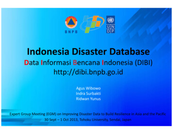
international conferences and international organisations. For example, the 2011Chengdu Declaration for Action states, ‘DRR was not expenditure but a no-regretinvestment that could protect lives, property, livelihoods, schools, businesses andemployment’ (UNDRR, 2011). In reference to this declaration, the Japan InternationalCooperation Agency (JICA) also stated that it ‘disseminates a concept of “low regretinvestment”, which is to make prior investment for DRR according to the assessmentof disaster risk and damage in order to make regret as small as possible, instead ofallocating budgets for recovery and reconstruction, and to adapt to future environmentchanges’ (JICA, n.d.).Although the importance of prior investments for DRR is recognisedinternationally, the budget allocated for these prior investments is still insufficient indeveloping countries. Figure 2 shows that prevention and preparedness activitiesaccount for only a few percent of disaster-related aid.Disaster-related Aid Commitments (US Thousand)Figure 2: Disaster-related Aid CommitmentsSources: Sudo (2019), World Bank (2013).In the Asian region, during the 7-year period from 2006 to 2012 in Indonesia andthe 7-year period from 2005 to 2011 in India, the yearly budget allocated to priorinvestments for DRR remained at an average of 0.1% of the gross domestic product(GDP) in each respective country (Chakrabarti and Prabodh, 2012; Darwanto, 2012;ESCAP, 2015). On the other hand, Japan, which has faced many large-scale disastersand has had a history of treating DRR measures with high regard, has allocated a yearlybudget at an average of 0.7% of their GDP to prior investments for DRR over 55 years3
spanning 1962 to 2016 (Government of Japan, Cabinet Office; Government of Japan,Ministry of Land, Infrastructure, Transport and Tourism; World Bank).One of the issues involved in implementing and facilitating DRR investmentpolicies in developing countries, including that of the Association of Southeast AsianNations (ASEAN) Community, is having the long-term impacts of natural disastersand the importance of DRR investment recognised by policymakers and treasurers inthe government, in addition to providing the support needed to make the appropriatedecisions. In order to make the appropriate decisions for DRR investment policies, itwould be effective to present information that provides answers for questions such as:‘What would be the maximum level of economic development to which the DRRinvestment is able to generate potentially?; What is the degree of economicdevelopment that is expected to be generated reliably from this?; What is the mostappropriate proportion of funds that should be allocated to the budget for the DRRinvestment?’; and ‘Can the budget that was invested in DRR be recovered reliably?Moreover, towards improving investment decision-making for DRR, severalsuggestions are presented for addressing the technical and political challenges: listingeconomic benefits and costs, listing key stakeholders and distributional economicimpacts, and learning from other economic assessments (Vorhies, 2012). The use ofeconomic models is an effective policy support tool to quantitatively presentinformation concerning the optimal level and economic efficiency of the DRRinvestment.There have been several past studies on economic models relating to naturaldisasters, DRR investments, and disaster finance. For example, such models includethe analytical framework for the design, pricing, and applications of index-based risktransfer products as a means to handle insurance market imperfections under disasterrisks in developing Asian countries (Chantarat et al., 2013), the regression model toshow that ex-ante cash transfer programs play a crucial role in encouraging poorhouseholds under the threat of disaster in Cambodia to invest in business rather thanin food (Vathana et al., 2013), the input–output (I–O) model to examine economiclosses and damages caused by natural disasters at the local, national, and the regionallevels in the ASEAN region (Shiomi, Ono, and Fukushima, 2019). Moreover, as auseful financial evaluation tool for DRR policies, there is the catastrophe simulation4
(CATSIM) model that made it possible to analyse, from the standpoint of financialstrategies, the vulnerabilities of a nation’s finances when faced with natural disasters(e.g. Mechler et al., 2006), as well as the endogenous business cycle model that madeit possible to analyse the long-term impacts of natural disasters on asset formation andproduction volume (e.g. Hallegatte, Hourcade, and Dumas, 2007; Hallegatte and Ghil,2008). By looking at the progression in which production capital and DRR capital areformed, a dynamic stochastic macroeconomic model that has made it possible toperform a qualitative analysis on long-term DRR investment policies is also cited (Segi,Ishikura, and Yokomatsu, 2012). Furthermore, in the study conducted by Yokomatsuet al. (2014), human capital was introduced into the dynamic stochasticmacroeconomic model, and the quantitative impact of DRR investments on theeconomic growth and social disparity of developing countries was also displayed.Additionally, by introducing policy variables for DRR investments and theaccumulation of DRR capital, the study conducted by Ishiwata and Yokomatsu (2018)was also able to quantitatively determine the optimal level of DRR investment thatshould be provided, in addition to demonstrating whether there was an ‘ex-ante riskreduction effect,’ which is an effect that is generated from DRR investments even whenno disasters have occurred. However, since the study conducted by Ishiwata andYokomatsu (2018) was a case study only on Pakistan, which has a history ofcatastrophic disasters such as floods, earthquakes, and droughts, in addition to havingthe socio-economic data required for numerical simulations such as the socialaccounting matrix and the household integrated economic survey, the extent of the exante risk reduction effect that would be generated in other developing countries, suchas those in the ASEAN, is still unclear.The purpose of this research is to analyse the way in which large-scale disastersas well as the presence or absence of DRR investments impact the economic growthof developing countries, including those of the ASEAN Community, on a long-termbasis. As a means of quantitatively analysing the optimal level and economicefficiency of DRR investments, a case study was conducted on Indonesia by utilisinga dynamic stochastic macroeconomic model that incorporates the idea of DRR.Through this method, the DRR investment policies operate in a quantitative manner,which then allowed us to make proposals for DRR investment policies, which were5
then analysed. The formulation of the model will be demonstrated in section 2, whichwill then lead into the deriving of the optimisation conditions in section 3, followedby the case study on Indonesia in section 4. Lastly, the conclusion andrecommendations of this research will be outlined in section 5.Model2.1. AssumptionsThe model used in this research is essentially a kind of the Ramsey growth model,which has a discrete time axis (Ramsey, 1928). This model also incorporates the addedvariables of disaster risk, DRR capital, and household assets. Although the research isbased on the model by Ishiwata and Yokomatsu (2018), the model assumes that humancapital is a constant variable throughout the calculation period, and it differs from theIshiwata and Yokomatsu model (2018) in that it takes into account the growth of thepopulation, enhancements in production technology, as well as the disaster damagerates and the depreciation rate of the DRR capital.The market is regarded as being completely competitive under the assumptionthat the economic space is a closed real economy that consists of one country that hasone sector. Whilst assuming that labour and production capital are necessarycomponents in the production of composite goods, it is also assumed that productionis carried out using the remaining factor of production in the event that some of thesecomponents are lost due to a disaster. In addition, rapid technological advancementsbrought about by changes to the socio-economic structure are viewed as unlikely tooccur.The representative household has an infinite time horizon and will undertakeeconomic activities in a completely rational manner with recognition of the disasterrisk. Based on the operation of real economics, the household income is treated asbeing equivalent to the production value, and it is also assumed that a certainpercentage of the household income is allocated to DRR investment every year.6
Under these assumptions, the model can be described as an Arrow–Debreweconomy, which achieves the Pareto-optimal allocation. Therefore, the solution of thecentral planning problem, in which the representative household allocates all theresources over an infinite time horizon to maximise its expected lifetime utility underits budget constraint, coincides with the solution of the market-oriented problem(Stokey, Lucas, and Prescott, 1989). Following most real business cycle models(Kydland and Prescott, 1982), the analysis is carried out under the framework of acentrally-planned economy where the solution can be generally derived more easilythan a market-oriented economy.2.2. Probability of Disaster Occurrence and the Damage RateAssuming that one disaster scale is determined in each period, the probability 𝜇 𝑙of a disaster with a disaster scale of 𝑙 {1,2, , 𝐿} occurring is constant regardless ofthe time, and it also satisfies 𝜇 𝑙 1.𝑙Superscript will be used to indicate the disaster scale 𝑙.There are four types of disaster damage rates: the labour supply damage rate𝜔𝑙 ( ) ; the household asset damage rate 𝜙 𝑙 ( ) ; the production capital damage rate𝜓𝑙 ( ); and the DRR capital damage rate 𝜎 𝑙 ( ). It is assumed that according to thedisaster damage mitigation function 𝜁𝓍 ( ), the disaster damage rates for each disasterscale 𝑙 will decrease as the DRR capital 𝑔(𝑡) accumulates:𝜔𝑙 (𝑔(𝑡)) 𝜔0𝑙 𝜁𝜔 (𝑔(𝑡)),Labour supply damage rate:Household asset damage rate:𝜙 𝑙 (𝑔(𝑡)) 𝜙0𝑙 𝜁𝜙 (𝑔(𝑡)),Production capital damage rate: 𝜓𝑙 (𝑔(𝑡)) 𝜓0𝑙 𝜁𝜓 (𝑔(𝑡)),𝜎 𝑙 (𝑔(𝑡)) 𝜎0𝑙 𝜁𝜎 (𝑔(𝑡))DRR capital damage rate:for all 𝑙, where 𝜔0𝑙 , 𝜙0𝑙 , 𝜓0𝑙 , and 𝜎0𝑙 respectively indicate the labour supply damage rate,the household asset damage rate, the production capital damage rate, and the DRRcapital damage rate in the base year. The functions of the production capital damage7
rate and the DRR capital damage rate have the modifiers of business continuity plansand insurance markets.It is assumed that a power function that has DRR capital 𝑔(𝑡) as its variable, isused for the disaster damage mitigation function 𝜁𝓍 ( ): 𝜈𝑥𝑔(𝑡)𝜁𝓍 (𝑔(𝑡)) []𝑔0,𝓍 {𝜔, 𝜙, 𝜓, 𝜎},where 𝜈𝑥 denotes the effect parameter of disaster damage mitigation, whereas 𝑔0denotes the accumulated DRR capital in the base year.2.3. Production Technology of Composite GoodsWhilst assuming that the Cobb–Douglas production function 𝑓( ) is used forcomposite goods, it is also assumed that composite goods are produced using the factorof production that remains after a disaster with the disaster scale of 𝑙 has occurred:𝛼ℎ𝛼𝑘𝑓 (𝐵(𝑡), ℎ̂𝑙 (𝑡), 𝑘̂ 𝑙 (𝑡)) 𝐵(𝑡)[ℎ̂𝑙 (𝑡)] [𝑘̂𝑙 (𝑡)]for all 𝑙, where𝐵(𝑡) 𝐵0 (1 𝛽)𝑡 𝑡0 ,ℎ̂𝑙 (𝑡) [1 𝜔𝑙 (𝑔(𝑡))]ℎ̅,𝑘̂ 𝑙 (𝑡) [1 𝜓𝑙 (𝑔(𝑡))]𝑘(𝑡),and𝛼𝑖 (0,1), 𝛼𝑖 1 ,𝑖 {ℎ,𝑘}where 𝐵(𝑡) denotes the total factor productivity (TFP), 𝐵0 denotes the TFP in the baseyear, 𝛽 denotes the TFP growth rate, 𝑡0 denotes the base year, and 𝛼𝑖 denotes the shareparameter of the components of production. Additionally, ℎ̅ denotes the human capitaland it is assumed that ℎ̅ 1.8
As with management of domestic economy and finance, GDP 𝐹 𝑙 (𝑡) isequivalent to the aggregate production value. Therefore, it can be expressed as followsby using the total population 𝑁(𝑡):𝐹 𝑙 (𝑡) 𝑁(𝑡) 𝑓 (𝐵(𝑡), ℎ̂𝑙 (𝑡), 𝑘̂ 𝑙 (𝑡))for all 𝑙, where𝑁(𝑡) 𝑁0 (1 𝑛)𝑡 𝑡0 ,where 𝑁0 denotes the total population in the base year, whilst 𝑛 denotes the populationgrowth rate.2.4. Economic Activities of a Householda)Maximising the Expected Lifetime UtilityWhen faced with disaster risk, the representative household allocates resourcesin a completely rational manner so as to maximise expected lifetime utility, which isdefined by the accumulated amount of non-durable goods consumption 𝑐 𝑙 (𝑡) andhousehold assets 𝓏(𝑡): Ε𝑙 [ 𝑢 (𝑐 𝑙 (𝑡′), 𝓏̂ 𝑙 (𝑡′)) 𝛬𝑡′ 𝑡],𝑡 ′ 𝑡where𝓏̂ 𝑙 (𝑡) [1 𝜙 𝑙 (𝑔(𝑡))]𝓏(𝑡),1𝛬 ,1 𝜌where Ε𝑙 [ ] is a symbol that denotes the expectation operator of the disaster scale 𝑙. Inaddition, 𝜌 refers to the time preference rate, whilst 𝛬 refers to the discount factor.9
The Stone–Geary utility function, which is able to express the situation in whichthe investments in each stock are not prioritised and the economic growth is stagnatedwhen the level of consumption is close to the subsistence level of consumption –namely, when the marginal utility of consumption is large – is used as the one-periodutility function 𝑢( ):𝑢(𝑐 𝑙 (𝑡), 𝓏̂ 𝑙 (𝑡)) 𝛾𝑐[𝑐 𝑙 (𝑡) 𝑐̅]1 𝜃𝑐 1[𝓏̂ 𝑙 (𝑡)]1 𝜃𝓏 1 𝛾𝓏1 𝜃𝑐1 𝜃𝓏for all 𝑙, whereγ𝑗 (0,1), 𝛾𝑗 1 ,𝑗 {𝑐,𝓏}where 𝛾𝑗 denotes the share parameter of consumption, 𝑐̅ denotes the minimumsubsistence level of consumption, and 𝜃𝑗 denotes the relative risk aversion. When theconsumption of non-durable goods 𝑐 𝑙 (𝑡)( 𝑐̅) approaches the minimum subsistencelevel of consumption𝑐̅, the marginal utility 𝑢( ) 𝑐 𝑙 (𝑡) of the consumption of nondurable goods increases, whilst the level of priority placed on allocating resources tothe consumption of non-durable goods 𝑐 𝑙 (𝑡) is heightened. As a result, there will be adelay in capital formation, which will in turn lead to a slowdown in economic growth.b)Accumulation of DRR CapitalThe DRR capital 𝑔(𝑡) serves the role of reducing each of the disaster damagerates. The progression of the accumulation of DRR capital is as follows.𝑔𝑙 (𝑡 1) (1 𝛿𝜎 𝑛)𝑔̂𝑙 (𝑡) 𝑑 𝑓 (𝐵(𝑡), ℎ̂𝑙 (𝑡), 𝑘̂ 𝑙 (𝑡))for all 𝑙 and 𝑑, where𝑔̂𝑙 (𝑡) [1 𝜎 𝑙 (𝑔(𝑡))]𝑔(𝑡),where 𝛿𝜎 denotes the depreciation rate of the DRR capital, whilst 𝑑 denotes theproportion of income that is allocated to the DRR investment. As the DRR capital 𝑔(𝑡)decreases at a constant rate (𝛿𝜎 𝑛) every year, only the DRR capital damage10
rate 𝜎 𝑙 ( ) is worsened due to disasters. However, at the same time, only new DRRinvestments are accumulated 𝑑 𝑓( ). In this model, although the DRR investment rate𝑑 is dealt with as a policy variable for the simplicity of calculation, based on the Solowgrowth model (Solow, 1956), if it is dealt with as an endogenous variable, based onthe Ramsey growth model (Ramsey, 1928), the scale of DRR investment 𝑑 𝑓( ) couldbe more linked to market forces, that is, the DRR investment rate 𝑑 would be larger indeveloped societies, and smaller in developing societies.Accumulation of Household Assetsc)Household assets 𝓏(𝑡) refer to durable goods such as houses and householdbelongings. The progression of the accumulation of household assets 𝓏(𝑡) is asfollows.𝓏 𝑙 (𝑡 1) (1 𝛿𝓏 𝑛)𝓏̂ 𝑙 (𝑡) 𝜉(𝑡)for all 𝑙 , where 𝛿𝓏 denotes the depreciation rate of household assets, whilst 𝜉(𝑡)denotes the household asset investment. As the household assets 𝓏(𝑡) decrease at aconstant rate (𝛿𝑧 𝑛) every year, only the household asset damage rate 𝜙 𝑙 ( ) isworsened due to disasters. However, at the same time, the amount of household assetinvestments 𝜉(𝑡) is newly accumulated.d)Accumulation of Production CapitalProduction capital 𝑘(𝑡) refers to infrastructure that is needed in productionprocess, such as production facilities or production equipment. The progression of theaccumulation of production capital 𝑘(𝑡) is as follows.𝑘 𝑙 (𝑡 1) (1 𝛿𝑘 𝑛)𝑘̂ 𝑙 (𝑡) (1 𝑑) 𝑓 (𝐵(𝑡), ℎ̂𝑙 (𝑡), 𝑘̂ 𝑙 (𝑡)) 𝑐 𝑙 (𝑡) 𝜉(𝑡)for all 𝑙 , where 𝛿𝑘 denotes the depreciation rate of the production capital. As theproduction capital 𝑘(𝑡) decreases at a constant rate (𝛿𝑘 𝑛) every year, only theproduction capital damage rate 𝜓𝑙 ( ) is worsened due to disasters. Additionally, theformation of production capital 𝑘(𝑡) progresses further as the consumption of non-11
durable goods 𝑐 𝑙 (𝑡) and household asset investment 𝜉(𝑡) decreases. This capitalformation in turn increases the production volume 𝑓( ) of composite goods andstimulates economic growth.e)Definition of Total AssetsTotal assets 𝑎(𝑡) is defined as the sum that is derived when household assets𝓏(𝑡) and production capital 𝑘(𝑡) are added together.𝑎𝑙 (𝑡 1) 𝓏 𝑙 (𝑡 1) 𝑘 𝑙 (𝑡 1) (1 𝛿𝓏 𝑛)𝓏̂ 𝑙 (𝑡) (1 𝛿𝑘 𝑛)𝑘̂𝑙 (𝑡) (1 𝑑) 𝑓 (𝐵(𝑡), ℎ̂𝑙 (𝑡), 𝑘̂ 𝑙 (𝑡)) 𝑐 𝑙 (𝑡) (1 𝛿𝓏 𝑛)𝓏̂ 𝑙 (𝑡) (1 𝛿𝑘 𝑛)[𝑎̂𝑙 (𝑡) 𝓏̆ 𝑙 (𝑡)] (1 𝑑) 𝑓 (𝐵(𝑡), ℎ̂𝑙 (𝑡), 𝑎̂𝑙 (𝑡) 𝓏̆ 𝑙 (𝑡)) 𝑐 𝑙 (𝑡)for all 𝑙 and 𝑑, where𝑎̂𝑙 (𝑡) [1 𝜓𝑙 (𝑔(𝑡))]𝑎(𝑡),𝓏̆ 𝑙 (𝑡) [1 𝜓 𝑙 (𝑔(𝑡))]𝓏(𝑡).By defining total assets 𝑎(𝑡), the household asset investment 𝜉(𝑡), which is oneof the control variables, is cancelled out. For this reason, household assets 𝓏(𝑡), whichis a state variable, as a control variable with respect to the total assets 𝑎(𝑡) can betreated; thus, making it convenient when calculations are made.12
3)Dynamic Optimisation3.1. Flow of EventsThe assumed flow of events in year 𝑡 is as follows.i)At the beginning of year 𝑡 , the representative household confirms theaccumulated amount of total assets 𝑎(𝑡) and DRR capital 𝑔(𝑡), along with theTFP 𝐵(𝑡), and the level of the DRR investment ratio 𝑑.ii)For the ex-ante problem, the representative household determines the level ofholding for household assets 𝓏(𝑡) in the year 𝑡 in order to maximise the expectedlifetime utility, of which the maximisation is achieved by the optimal allocationof consumption and investments in each stock throughout present and futureperiods, when faced with a disaster risk. In addition, the level of holding forproduction capital 𝑘(𝑡) 𝑎(𝑡) 𝓏(𝑡) is also determined through this.iii)A disaster with a disaster scale of 𝑙 occurs, leading to a loss in each type ofcapital, which corresponds to disaster damage rates. Household assets 𝓏(𝑡) ,production capital 𝑘(𝑡), and DRR capital 𝑔(𝑡) will be subjected to continuedmultiplicative shocks, whilst the labour supply ℎ̅ will be subjected to temporarymultiplicative shocks.iv)For the ex-post problem, composite goods will be produced from the remainingcomponents of production, whilst the representative household goes on to earnan income 𝑓( ) . A portion of this income will be allocated to the DRRinvestment 𝑑 𝑓( ). At the same time, the consumption of non-durable goods𝑐 𝑙 (𝑡) will be determined, alongside the instant utility level 𝑢( ).v)At the end of year 𝑡, the total assets 𝑎𝑙 (𝑡 1) of year 𝑡 1, the DRR capital𝑔𝑙 (𝑡 1), as well as the TFP 𝐵(𝑡 1) will be determined. Afterwards, the samecycle will be repeated from i).3.2. Value FunctionThe representative household’s issue with dynamic optimisation is described asfollows by using the value function 𝑉( ) under the constraints of the formation of eachtype of capital.13
𝑉(𝑎(𝑡), 𝑔(𝑡), 𝐵(𝑡), 𝑑) max E𝑙 [ 𝑢 (𝑐 𝑙 (𝑡 ′ ) , 𝓏̂ 𝑙 (𝑡 ′ )) 𝛬𝑡′ 𝑡],𝑡 ′ 𝑡s.t.𝑎𝑙 (𝑡 1) (1 𝛿𝓏 𝑛)𝓏̂ 𝑙 (𝑡) (1 𝛿𝑘 𝑛)[𝑎̂𝑙 (𝑡) 𝓏̆ 𝑙 (𝑡)] (1 𝑑) 𝑓 (𝐵(𝑡), ℎ̂𝑙 (𝑡), 𝑎̂𝑙 (𝑡) 𝓏̆ 𝑙 (𝑡)) 𝑐 𝑙 (𝑡),𝑔𝑙 (𝑡 1) (1 𝛿𝜎 𝑛)𝑔̂(𝑡) 𝑑 𝑓 (𝐵(𝑡), ℎ̂𝑙 (𝑡), 𝑎̂𝑙 (𝑡) 𝓏̆ 𝑙 (𝑡)),𝑎𝑙 (𝑡 1), 𝑔𝑙 (𝑡 1) 0for all 𝑙 and 𝑑. The value function 𝑉( ) can be regarded as an index of social welfareas it is the maximum value of the expected utility function that can be achieved throughthe optimal allocation of resources.The equation above is equivalent to the Bellman equation (Bellman, 1957)shown below, which is a recursive equation:𝑉(𝑎(𝑡), 𝑔(𝑡), 𝐵(𝑡), 𝑑) 𝑙 max E𝑙 [𝑢(𝑐 𝑙 (𝑡), 𝓏̂ 𝑙 (𝑡)) 𝛬 𝑉(𝑎𝑙 (𝑡 1), 𝑔𝑙 (𝑡 1), 𝐵(𝑡 1), 𝑑)]𝑐 (𝑡),.𝓏(𝑡) 𝑙 max 𝜇 𝑙 [𝑢(𝑐 𝑙 (𝑡), 𝓏̂ 𝑙 (𝑡)) 𝛬𝑐 (𝑡),.𝓏(𝑡)𝑙 𝑉(𝑎𝑙 (𝑡 1), 𝑔𝑙 (𝑡 1), 𝐵(𝑡 1), 𝑑)] .3.3. Optimal ConditionsThe first-order conditions for the consumption of non-durable goods 𝑐 𝑙 (𝑡) andhousehold assets 𝓏(𝑡) , with regards to the value function 𝑉( ) described by theBellman equation, is as follows.𝑐 𝑙 (𝑡) 𝑢𝑐𝑙 (𝑡) 𝛬 𝑉𝑎𝑙 (𝑡 1)𝓏(𝑡) 𝜇𝑙𝑙[𝑢𝑧𝑙 (𝑡) 𝛬 {𝑉𝑎𝑙 (𝑡for all 𝑙, 𝑎𝑙 (𝑡 1) 𝑔𝑙 (𝑡 1)𝑙 (𝑡 1) 𝑉𝑔 1) }] 0, 𝓏(𝑡) 𝓏(𝑡)14
where 𝑉(𝑎𝑙 (𝑡 1), 𝑔𝑙 (𝑡 1), 𝐵(𝑡 1), 𝑑) 1) , 𝑎𝑙 (𝑡 1) 𝑉(𝑎𝑙 (𝑡 1), 𝑔𝑙 (𝑡 1), 𝐵(𝑡 1), 𝑑)𝑉𝑔𝑙 (𝑡 1) , 𝑔𝑙 (𝑡 1)𝑉𝑎𝑙 (𝑡𝑢𝑐𝑙 (𝑡)𝑢𝑧𝑙 (𝑡) 𝑢(𝑐 𝑙 (𝑡), 𝓏̂ 𝑙 (𝑡)) 𝑐 𝑙 (𝑡), 𝑢(𝑐 𝑙 (𝑡), 𝓏̂ 𝑙 (𝑡)) 𝓏(𝑡)for all 𝑑. The first-order conditions for the consumption of non-durable goods 𝑐 𝑙 (𝑡)show that the marginal utility of the consumption of non-durable goods 𝑐 𝑙 (𝑡) isequivalent to the marginal value of the present discount factor for total assets 𝑎(𝑡).The transversality conditions, which are the complementary conditions for theend of a period, are as follows. 𝑉(𝑎(𝑡), 𝑔(𝑡), 𝐵(𝑡), 𝑑) 𝑡 𝛬 0,𝑡 𝑎(𝑡) 𝑉(𝑎(𝑡), 𝑔(𝑡), 𝐵(𝑡), 𝑑) 𝑡lim 𝑔(𝑡) 𝛬 0 for all 𝑑.𝑡 𝑔(𝑡)lim 𝑎(𝑡) In this research, the value function expressed by the Bellman equation is used asan objective function. Under the constraints of the formation of each type of capital,this objective function is then solved via a numerical simulation method called ValueFunction Iteration (e.g. Heer and Maußner, 2008), which allows us to numericallyobtain the socially optimal solution.15
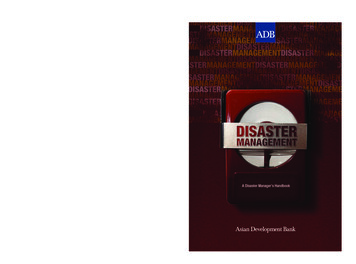
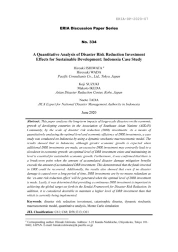
4.Case Study: Effects of DRR Investments in Indonesia4.1. Prerequisites of the SettingA case study was conducted in Indonesia to demonstrate quantitatively that DRRinvestments are indispensable to the economic and social development of developingcountries, including those of the ASEAN Community. Indonesia has the largestaverage annual loss amongst the ASEAN Community, as shown in Figure 3, and alsooften faces catastrophic disasters such as the 2004 Indian Ocean and the 2018 Sulawesiearthquake and tsunami. With 2003 as its base year, the case study was conducted overa total estimated period of 28 years spanning 2003 to 2030. Furthermore, economicgrowth was calculated on a yearly interval.Figure 3: Average Annual Loss for Different Countries and the ASEAN Region,1970 to 2009AAL (in US 84272205AAL average annual loss, ASEAN Association of Southeast Asian Nations.Source: Adapted from Gupta (2010).The parameter values used in this case study are listed in Tables A1 and A2 (seeAppendix). Some of the parameter values were set using assumed values due to therestrictions on matters such as the amount of data that can be stored in Indonesia. Forexample, for the effect parameter of disaster damage mitigation 𝜈𝑥 in the disasterdamage mitigation function 𝜁𝓍 ( ), estimates from data such as flood damage statisticsand social capital stock figures, etc. in Japan for the period between 1953 and 2014were used, since there was only around 10 years’ worth of data for that period inIndonesia and precisely estimating the function was difficult. These assumed values16
will need to be replaced in the future once data has been accumulated for the countrywhere the case study is conducted.Data on the socio-economics of Indonesia was mainly sourced from the 2003Social Accounting Matrix created by Yusuf (2006), as well as the World DevelopmentIndicators, which is the statistics database of the World Bank. Using this data, theinitial value of each state variable and calibrated parameter value in the base year wasestablished.Data on the disaster damage in Indonesia was sourced from disaster statistics bythe Indonesian National Agency for Disaster Countermeasure (BNPB). However,given inadequacies in the data accuracy of older disaster damage data sets, eachdisaster damage rate was estimated using data from 2002 to 2016, which is the periodof 15 years where a relatively large amount of data on disaster damage was recorded.Out of all the natural disasters that occurred during the aforementioned period, flooddamage (floods, tsunamis,1 storm surges, landslides) made up around 61.1% of thenumber of disaster records. Flood damage was also the reason for around 99.3% of theeconomic loss sustained, and it was attributable for a majority of around 79.5% of thenumber of disaster victims (dead, injured, missing, evacuees, and those affected bydisasters) (according to the disaster statistics provided by BNPB). For these reasons,‘flood damage’ was chosen as the disaster to be covered in the case study. In this casestudy, the disaster damage rates for each type of capital is classified into five ranks,whereby disaster scale 𝑙 1 is defined as the lowest level of disaster damage, anddisaster scale 𝑙 5 is defined as the highest level of disaster damage. However, asthere is only a small number of inter-annual disaster records that can be used toestimate the disaster damage rates by disaster scales, the average value for the amountof damage sustained each year from disasters is assumed to be Rp30 trillion (BNPB,2016), which is the figure that was published by the BNPB in Indonesia. Subsequently,this average value along with the data on disaster damage for each year is used toderive the standard deviation of the amount of disaster damage sustained. Followingthis, the disaster damage rates for each disaster scale is then determined by looking atIt is important to note that the damage caused by the 2004 Indian Ocean earthquake, which struck offthe coast of Sumatra, is recorded as the sum of the damages sustained from both the tsunami andearthquake. Therefore, the figure for the damage caused by the tsunami also incorporates the damagecaused by the earthquake.117
the discrepancies with the average value. These disaster damage rates will need to beimproved in the future once data has been accumulated and must be accurate for thecountry where the case study is conducted – in this case, Indonesia. Although the setvalues of the disaster damage rates are not 0% for the disaster scale 𝑙 1, the valuesare still very small. Therefo
A Quantitative Analysis of Disaster Risk Reduction Investment Effects for Sustainable Development: Indonesia Case Study Hiroaki ISHIWATA Hiroyuki WADA Pacific Consultants Co., Ltd., Tokyo, Japan Koji SUZUKI Makoto IKEDA Asian Disaster Reduction Center, Kobe, Japan Naoto TADA JICA Exper