Transcription
Introduction to Nonlinear RegressionAndreas Ruckstuhl IDP Institut für Datenanalyse und ProzessdesignZHAW Zürcher Hochschule für Angewandte Wissenschaften2016†Contents1. Estimation and Standard Inference21.1. The Nonlinear Regression Model . . . . . . . . . . . . . . . . . . . . . . 21.2. Model Fitting Using an Iterative Algorithm . . . . . . . . . . . . . . . . 61.3. Inference Based on Linear Approximations . . . . . . . . . . . . . . . . . 122. Improved Inference and Its Visualisation2.1. Likelihood Based Inference . . . . .2.2. Profile t-Plot and Profile Traces . . .2.3. Parameter Transformations . . . . .2.4. Bootstrap . . . . . . . . . . . . . . .18182022293. Prediction and Calibration333.1. Prediction . . . . . . . . . . . . . . . . . . . . . . . . . . . . . . . . . . . 333.2. Calibration . . . . . . . . . . . . . . . . . . . . . . . . . . . . . . . . . . 354. Closing Comments37A. Appendix38A.1. The Gauss-Newton Method . . . . . . . . . . . . . . . . . . . . . . . . . 38 †E-Mail Address: Andreas.Ruckstuhl@zhaw.ch; Internet: http://www.idp.zhaw.chThe author thanks Werner Stahel for his valuable comments and Amanda Strong and Lukas Meierfor their help in translating the original German version into English.1
Contents1GoalsThe nonlinear regression model block in the Weiterbildungslehrgang (WBL) in angewandter Statistik at the ETH Zurich should1. introduce problems that are relevant to the fitting of nonlinear regression functions,2. present graphical representations for assessing the quality of approximate confidence intervals, and3. introduce some parts of the statistics software R that can help with solvingconcrete problems.A. Ruckstuhl, ZHAW
1. Estimation and Standard Inference1.1. The Nonlinear Regression ModelaThe Regression Model. Regression studies the relationship between a variable ofinterest Y and one or more explanatory or predictor variables x(j) . The generalmodel is(1) (2)(m)Yi hhxi , xi , . . . , xi ; θ1 , θ2 , . . . , θp i Ei .Here, h is an appropriate function that depends on the predictor variables and(1) (2)(m)parameters, that we want to combine into vectors x [xi , xi , . . . , xi ]T andθ [θ1 , θ2 , . . . , θp ]T . We assume that the errors are all normally distributed andindependent, i.e.DEEi N 0, σ 2 , independent.bThe Linear Regression Model. In (multiple) linear regression, we considered functionsh that are linear in the parameters θj ,(1)(2)(m)hhxi , xi , . . . , xi(1)(2); θ1 , θ2 , . . . , θp i θ1 xei θ2 xei(p) . . . θp xei ,where the xe(j) can be arbitrary functions of the original explanatory variables x(j) .There the parameters were usually denoted by βj instead of θj .c The Nonlinear Regression Model. In nonlinear regression, we use functions h thatare not linear in the parameters. Often, such a function is derived from theory. Inprinciple, there are unlimited possibilities for describing the deterministic part of themodel. As we will see, this flexibility often means a greater effort to make statisticalstatements.Example dPuromycin The speed of an enzymatic reaction depends on the concentration of asubstrate. As outlined in Bates and Watts (1988), an experiment was performed toexamine how a treatment of the enzyme with an additional substance called Puromycininfluences the reaction speed. The initial speed of the reaction is chosen as the responsevariable, which is measured via radioactivity (the unit of the response variable iscount/min 2 ; the number of registrations on a Geiger counter per time period measuresthe quantity of the substance, and the reaction speed is proportional to the change pertime unit).The relationship of the variable of interest with the substrate concentration x (in ppm)is described by the Michaelis-Menten functionhhx; θi 2θ1 x.θ2 x
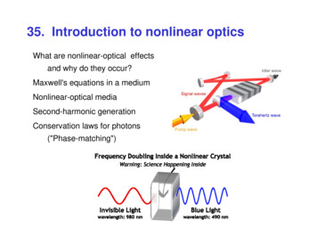
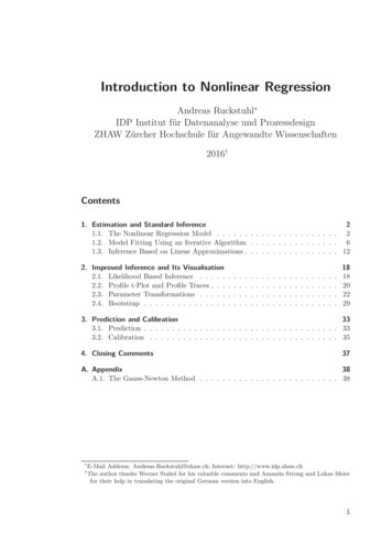
1.1. The Nonlinear Regression 0ConcentrationConcentrationFigure 1.1.d.: Puromycin. (a) Data ( treated enzyme; untreated enzyme) and (b) typicalshape of the regression function.An infinitely large substrate concentration (x ) leads to the “asymptotic” speedθ1 . It was hypothesized that this parameter is influenced by the addition of Puromycin.The experiment is therefore carried out once with the enzyme treated with Puromycinand once with the untreated enzyme. Figure 1.1.d shows the result. In this sectionthe data of the treated enzyme is used.Example e Biochemical Oxygen Demand To determine the biochemical oxygen demand, streamwater samples were enriched with soluble organic matter, with inorganic nutrientsand with dissolved oxygen, and subdivided into bottles (Marske, 1967, see Bates andWatts, 1988). Each bottle was inoculated with a mixed culture of microorganisms,sealed and put in a climate chamber with constant temperature. The bottles wereperiodically opened and their dissolved oxygen concentration was analyzed, from whichthe biochemical oxygen demand [mg/l] was calculated. The model used to connect thecumulative biochemical oxygen demand Y with the incubation time x, is based onexponential decay: h hx; θi θ1 1 e θ2 x .Figure 1.1.e shows the data and the regression function.Example fMembrane Separation Technology (Rapold-Nydegger, 1994). The ratio of protonatedto deprotonated carboxyl groups in the pores of cellulose membranes depends on thepH-value x of the outer solution. The protonation of the carboxyl carbon atoms canbe detected by 13 C-NMR. We assume that the relationship can be described by theextended “Henderson-Hasselbach Equation” for polyelectrolyteslog10θ1 yy θ2 θ3 θ4 x ,where the unknown parameters are θ1 , θ2 and θ3 0 and θ4 0. Solving for y leadsto the modelθ1 θ2 10θ3 θ4 xiYi hhxi ; θi Ei Ei .1 10θ3 θ4 xiThe regression function hhxi , θi for a reasonably chosen θ is shown in Figure 1.1.f nextto the data.A. Ruckstuhl, ZHAW
41.1. The Nonlinear Regression Model20Oxygen DemandOxygen Demand181614121081234567DaysDaysFigure 1.1.e.: Biochemical Oxygen Demand. (a) Data and (b) typical shape of the regressionfunction.162yy ( chem. shift)163161160(a)246810(b)12xx ( pH)Figure 1.1.f.: Membrane Separation Technology. (a) Data and (b) a typical shape of the regres-sion function.gSome Further Examples of Nonlinear Regression Functions. Hill model (enzyme kinetics): hhxi , θi θ1 xθi 3 /(θ2 xθi 3 )For θ3 1 this is also known as the Michaelis-Menten model (1.1.d). Mitscherlich function (growth analysis): hhxi , θi θ1 θ2 exphθ3 xi i. From kinetics (chemistry) we get the function(1)(2)(1)(2)hhxi , xi ; θi exph θ1 xi exph θ2 /xi ii. Cobbs-Douglas production functionD(1)(2)h xi , xi ; θE θ1 (1) θ2xi (2) θ3xi.Since useful regression functions are often derived from the theoretical background ofthe application of interest, a general overview of nonlinear regression functions is ofWBL Applied Statistics — Nonlinear Regression
1.1. The Nonlinear Regression Model5very limited benefit. A compilation of functions from publications can be found inAppendix 7 of Bates and Watts (1988).hTransformably Linear Regression Functions. Some nonlinear regression functionshave a very favourable structure. For example, a power functionh hx; θi θ1 xθ2can be transformed to a linear model by expressing the logarithm of h hx; θi as alinear (in the parameters) function of the logarithm of the explanatory variable xlnhh hx; θii ln hθ1 i θ2 ln hxi β0 β1 xe ,where β0 ln hθ1 i, β1 θ2 and xe ln hxi. We call such a regression function htransformably linear.i The Statistically Complete Model. The “regression fitting” of the “linearized” regression function given in the previous paragraph is based on the modellnhYi i β0 β1 xei Ei ,where the random errors Ei all have the same normal distribution. We transform thismodel back and getYi θ1 · xθ2 · Ee i ,with Ee i exphEi i. The errors Ee i , i 1, . . . , n, now have a multiplicative effect andare log-normally distributed! The assumption about the random errors is now clearlydifferent than for a regression model based directly on h,Yi θ1 · xθ2 Ei ,where the random error Ei contributes additively and is normally distributed.A linearization of the regression function is therefore advisable only if the assumptionsabout the random errors can be better satisfied – in our example, if the errors actuallyact multiplicatively rather than additively and are log-normally rather than normallydistributed. These assumptions must be checked with residual analysis (see,e.g., Figure1.1.i).j* Note:In linear regression it has been shown that the variance can be stabilized with certaintransformations (e.g. logh·i, · ). If this is not possible, in certain circumstances one can alsoperform a weighted linear regression. The process is analogous in nonlinear regression.A. Ruckstuhl, ZHAW
61.2. Model Fitting Using an Iterative Algorithm1000500ln(y) ln(a) b*ln(x) E 5000resid(SD2.nls)0.50.0 0.5 1.0resid(SD1.nls)nls(y a * x b)y a * x b E02004006008000200400800 1000fitted(SD2.nls)0.50.0resid(SD2.lm) 1.0 0.50.0 0.4 0.8 1.2resid(SD1.lm)lm(log(y) log(x))1.0fitted(SD1.nls)600 20246 20fitted(SD1.lm)246fitted(SD2.lm)Figure 1.1.i.: Tukey-Anscombe plots of four different situations. In the left column, the dataare simulated from an additive error model, whereas in the right column the data are simulatedfrom a multiplicative error model. The top row shows the Tukey-Anscombe plots of fits of amultiplicative error model to both data sets and the bottom row shows the Tukey-Anscombeplots of fits of an additive error model to both data sets.k Here are some more linearizable functions (see also Daniel and Wood, 1980):h hx; θi 1/(θ1 θ2 exph xi) h hx; θi θ1 x/(θ2 x) 1/h hx; θi 1/θ1 θ2 /θ1 x1h hx; θi θ1 xθ2 lnhh hx; θii lnhθ1 i θ2 lnhxi lnhh hx; θii lnhθ1 i θ2 ghxih hx; θi θ1 exphθ2 ghxiih hx; θi exph θ1 xh hx; θi θ1 x(1)(1) θ2exph θ2 /xx(2) θ3(2)ii 1/h hx; θi θ1 θ2 exph xilnhlnhh hx; θiii lnh θ1 i lnhx(1) i θ2 /x(2) lnhh hx; θii lnhθ1 i θ2 lnhx(1) i θ3 lnhx(2) i .The last one is the Cobbs-Douglas Model from 1.1.g.l We have almost exclusively seen regression functions that only depend on one predictorvariable x. This was primarily because it was possible to graphically illustrate themodel. The following theory also works well for regression functions h hx; θi thatdepend on several predictor variables x [x(1) , x(2) , . . . , x(m) ].1.2. Model Fitting Using an Iterative AlgorithmaThe Principle of Least Squares. To get estimates for the parameters θ [θ1 , θ2 , . . .,θp ]T , one applies – like in linear regression – the principle of least squares. The sumWBL Applied Statistics — Nonlinear Regression
1.2. Model Fitting Using an Iterative Algorithm7of the squared deviationsS(θ) : nX(yi ηi hθi)2where ηi hθi : hhxi ; θii 1should be minimized. The notation that replaces hhxi ; θi with ηi hθi is reasonablebecause [xi , yi ] is given by the data and only the parameters θ remain to be determined.Unfortunately, the minimum of S(θ) and thus the estimater have no explicit solutionas it was the case for linear regression. Iterative numeric procedures are thereforeneeded. We will sketch the basic ideas of the most common algorithm. It is also thebasis for the easiest way to derive tests and confidence intervals.bGeometrical Illustration. The observed values Y [Y1 , Y2 , . . . , Yn ]T define apoint in n-dimensional space. The same holds true for the “model values” η hθi [η1 hθi , η2 hθi , . . . , ηn hθi]T for a given θ .Please take note: In multivariate statistics where an observation consists of m variablesx(j) , j 1, 2, . . . , m, it’s common to illustrate the observations in the m-dimensionalspace. Here, we consider the Y - and η -values of all n observations as points in then-dimensional space.Unfortunately, geometrical interpretation stops with three dimensions (and thus withthree observations). Nevertheless, let us have a look at such a situation, first for simplelinear regression.c As stated above, the observed values Y [Y1 , Y2 , Y3 ]T determine a point in threedimensional space. For given parameters β0 5 and β1 1 we can calculate the modelvalues ηi β β0 β1 xi and represent the corresponding vector η β β0 1 β1 xas a point. We now ask: Where are all the points that can be achieved by varyingthe parameters? These are the possible linear combinations of the two vectors 1 andx and thus form the plane “spanned by 1 and x”. By estimating the parametersaccording to the principle of least squares, the squared distance between Y and η βis minimized. So, we want the point on the plane that has the least distance to Y .This is also called the projection of Y onto the plane. The parameter values thatcorrespond to this point ηb are therefore the estimated parameter values βb [βb0 , βb1 ]T .An illustration can be found in Figure 1.2.c.dNow we want to fit a nonlinear function, e.g. h hx; θi θ1 exp h1 θ2 xi, to the samethree observations. We can again ask ourselves where are all the points η hθi thatcan be achieved by varying the parameters θ1 and θ2 . They lie on a two-dimensionalcurved surface (called the model surface in the following) in three-dimensional space.The estimation problem again consists of finding the point ηb on the model surface thatis closest to Y . The parameter values that correspond to this point ηb are then theestimated parameter values θb [θb1 , θb2 ]T . Figure Figure 1.2.d illustrates the nonlinearcase.Example e Biochemical Oxygen Demand (cont’d) The situation for our Biochemical OxygenDemand example can be found in Figure 1.2.e. Basically, we can read the estimatedparameters directly off the graph here: θb1 is a bit less than 21 and θb2 is a bit largerthan 0.6. In fact the (exact) solution is θb [20.82, 0.6103] (note that these are theparameter estimates for the reduced data set only consisting of three observations).A. Ruckstuhl, ZHAW
81.2. Model Fitting Using an Iterative Algorithm10Y10Y6η 3 y386[1,1,1]864η3 y324200002468η2 y24102[1,1,1]810010x24xη2 y268y024η 1 y16810η 1 y1Figure 1.2.c.: Illustration of simple linear regression. Values of η β β0 β1 x for varyingparameters [β0 , β1 ] lead to a plane in three-dimensional space. The right plot also shows thepoint on the surface that is closest to Y [Y1 , Y2 , Y3 ]. It is the fitted value yb and determinesthe estimated parameters βb.1214η2 y2161820Y2120η 3 y319 102218567891011η1 y1Figure 1.2.d.: Geometrical illustration of nonlinear regression. The values of η hθi h hx; θ1 , θ2 ifor varying parameters [θ1 , θ2 ] lead to a two-dimensional “model surface” in three-dimensionalspace. The lines on the model surface correspond to constant η1 and η3 , respectively.WBL Applied Statistics — Nonlinear Regression
1.2. Model Fitting Using an Iterative Algorithm920θ1 22Yθ1 21θ1 20y18θ2 0.514η2 y2160.4120.3212019 102218η3 y3567891011η1 y1Figure 1.2.e.: Biochemical Oxygen Demand: Geometrical illustration of nonlinear regression.In addition, we can see here theD linesE of constant θ1 and θ2 , respectively. The vector of thebestimated model values yb h x; θ is the point on the model surface that is closest to Y .fApproach for the Minimization Problem. The main idea of the usual algorithm forminimizing the sum of squares (see 1.2.a) is as follows: If a preliminary best value θ(ℓ)exists, we approximatesurface with the plane that touches the surface atDD the modelEE(ℓ)(ℓ)the point η θ h x; θ(tangent plane). Now we are looking for the point onthat plane that lies closest to Y . This is the same as estimation in a linear regressionproblem. This new point lies on the plane, but not on the surface that corresponds tothe nonlinear problem. However, it determines a parameter vector θ(ℓ 1) that we useas starting value for the next iteration.gLinear Approximation. To determine the tangent plane we need the partial derivatives(j)Ai hθi : ηi hθi, θjthat can be summarized by an n p matrix A . The approximation of the modelsurface ηhθi by the tangent plane at a parameter value θ is(1)(p)ηi hθi ηi hθ i Ai hθ i (θ1 θ1 ) . Ai hθ i (θp θp )A. Ruckstuhl, ZHAW
101.2. Model Fitting Using an Iterative Algorithmor, in matrix notation,ηhθi ηhθ i A hθ i (θ θ ) .If we now add a random error, we get a linear regression modelYe A hθ i β Ewith “preliminary residuals” Ye i Yi ηi hθ i as response variable, the columns of Aas predictors and the coefficients βj θj θj (a model without intercept β0 ).hGauss-Newton Algorithm. The Gauss-Newton algorithm starts with an initial valueθ(0) for θ , solving the just introduced linear regression problem for θ θ(0) to find acorrection β and hence an improved value θ (1) θ(0) β . Again, the approximatedDmodel is calculated, and thus the “preliminary residuals” Y η θ(1)DEEand the partialderivatives A θ(1) are determined, leading to θ2 . This iteration step is continueduntil the the correction β is small enough. (Further details can be found in AppendixA.1.)It can not be guaranteed that this procedure actually finds the minimum of the sum ofsquares. The better the p-dimensional model surface at the minimum θb (θb1 , . . . , θbp )Tcan be locally approximated by a p-dimensional plane and the closer the initial valueθ(0) is to the solution, the higher are the chances of finding the optimal value.* Algorithms usually determine the derivative matrixA numerically. In more complex problems thenumerical approximation can be insufficient and cause convergence problems. For such situationsit is an advantage if explicit expressions for the partial derivatives can be used to determine thederivative matrix more reliably (see also Section 2.3).i Starting Values. An iterative procedure always requires a starting value. Good starting values help to find a solution more quickly and more reliably.Several simple but useful principles for determining starting values can be used: use prior knowledge; interpret the behavior of the expectation function h hi in terms of the parametersanalytically or graphically; transform the expectation function h hi analytically to obtain linear behavior; reduce dimensionality by substituting values for some parameters or by evaluating the function at specific design values; and use conditional linearity.jStarting Value from Prior Knowledge. As already noted in the introduction, nonlinearmodels are often based on theoretical considerations of the corresponding applicationarea. Already existing prior knowledge from similar experiments can be used to geta starting value. To ensure the quality of the chosen starting value, it is advisableto graphically represent the regression function hhx; θi for various possible startingvalues θ θ 0 together with the data (e.g., as in Figure 1.2.k, right).WBL Applied Statistics — Nonlinear Regression
110.0202000.015150Velocity1/velocity1.2. Model Fitting Using an Iterative ration0.40.60.81.0ConcentrationFigure 1.2.k.: Puromycin. Left: Regression function in the linearized problem. Right: Re-gression function hhx; θi for the starting values θ θ (0) (estimation θ θb (——–).) and for the least squaresk Starting Values From Transform the Expectation Function. Often – because of thedistribution of the error term – one is forced to use a nonlinear regression functioneven though the expectation function h hi cpuld be transformed to a linear function.However, the linearized expectation function can be used to get starting values.In the Puromycin example the regression function is linearizable: The reciprocal valuesof the two variables fulfill111θ2 1ye β0 β1 xe .yhhx; θiθ1 θ1 xThe least squares solution for this modified problem is βb [βb0 , βb1 ]T (0.00511, 0.000247)T(Figure 1.2.k, left). This leads to the starting values(0)θ1 1/βb0 196,(0)θ2 βb1 /βb0 0.048.l Starting Values from Interpreting the Behavior of h hi. It is often helpful to considerthe geometrical features of the regression function.In the Puromycin Example we can derive a starting value in another way: θ1 is theresponse value for x . Since the regression function is monotonically increasing, we(0)can use the maximal yi -value or a visually determined “asymptotic value” θ1 207as starting value for θ1 . The parameter θ2 is the x-value, such that y reaches half of(0)the asymptotic value θ1 . This leads to θ2 0.06.The starting values thus result from a geometrical interpretation of the parametersand a rough estimate can be determined by “fitting by eye”.Example mMembrane Separation Technology (cont’d) In the Membrane Separation Technologyexample we let x , so hhx; θi θ1 (since θ4 0); for x , hhx; θi θ2 .From Figure 1.1.f (a) we see that θ1 163.7 and θ2 159.5. Once we know θ1 andθ2 , we can linearize the regression function byye : log10*(0)θ1 y(0)y θ2 θ3 θ4 x .A. Ruckstuhl, ZHAW
121.3. Inference Based on Linear Approximations2(a)y ( Verschiebung)163y10 1162161160(b) 22468101224x ( pH)681012x ( pH)Figure 1.2.m.: Membrane Separation Technology. (a) Regression line that is used for determining the starting values for θ3 and θ4 . (b) Regression function hhx; θi for the starting value) and for the least squares estimator θ θb (——–).θ θ(0) (This is called conditional linearity of the expectation function. The linear regression(0)(0)model leads to the starting values θ3 1.83 and θ4 0.36, respectively.With this starting value the algorithm converges to the solution θb1 163.7, θb2 b are shown in159.8, θb3 2.675 and θb4 0.512. The functions hh·; θ (0) i and hh·; θiFigure 1.2.m (b).* Theproperty of conditional linearity of a function can also be useful to develop an algorithmspecifically suited for this situation (see e.g. Bates and Watts, 1988).nSelf-Starter Function. For repeated use of the same nonlinear regression modelsome automated way of providing starting values is demanded nowadays. Basically,we should be able to collect all the manual steps which are necessary to obtain theinitial values for a nonlinear regression model into a function, and use it to generatethe starting values. Such a function is called a self-starter function and should allowto run the estimating procedure easily and smoothly.Self-starter functions are specific for a given mean function and calculate starting valuesfor a given dataset. The challenge is to design a self-starter function robustly. That is,its resulting values must allow the estimation algorithm to converge to the parameterestimates.One of the self-starter knowledge bases comes with the standard installation of R. Youfind an overview in Table 1.2.n and some more details, including informations how towriter a self-starter yourself, in Ritz and Streibig (2008).1.3. Inference Based on Linear ApproximationsaThe estimator θb is the value of θ that optimally fits the data. We now ask whichparameter values θ are compatible with the observations. The confidence region isthe set of all these values. For an individual parameter θj the confidence region is aconfidence interval.These concepts have been discussed in great detail in the modul “Linear RegressionWBL Applied Statistics — Nonlinear Regression
1.3. Inference Based on Linear ApproximationsModel13Mean Functionlrc1A1 · e x·eBiexponentialAsymptotic regressionName of Self-Starter Functionlrc2 A2 · e x·eSSbiexp(x, A1, lrc1, A2, lrc2)lrcAsym (R0 Asym) · e x·elrcSSasymp(x, Asym, R0, lrc)Asymptotic regressionwith offsetAsymptotic regression(c0 0)First-ordercompartmentAsym · (1 e (x c0)·e )x1 · e elKa elKelKelKa·(e x2·e e x2·e )SSfol(x1, x2, lKe, lKa, lCl)GompertzAsym · e b2·b3xSSgompertz(x, Asym, b2, b3)LogisticLogistic (A 0)Michaelis-MentenWeibulllrcAsym · (1 e x·e)SSasympOrig(x, Asym, lrc)lKe lKa lClA B ASSfpl(x, A, B, xmid, scal)1 e(xmid x)/scalAsymSSlogis(x, Asym, xmid, scal)1 e(xmid x)/scalxV m · K xAsym Drop · eSSasympOff(x, Asym, lrc, c0)SSmicmen(x, Vm, K) elrc ·xpwrSSweibull(x, Asym, Drop, lrc, pwr)Table 1.2.n.: Available self-starter functions for nls() which come with the standard installationof R.Analysis”. As a look on the summary output of a nls object shows, it look very similarto the summary output of a fitted linear regression model.Example bMembrane Separation Technology (cont’d) The R summary output for the Membrane Separation Technology example can be found in Table 1.3.b. The parameterestimates are in column Estimate, followed by the estimated approximate standarderror (Std. Error) and the test statistics (t value), that are approximately tn pdistributed. The corresponding p-values can be found in column Pr( t ). The estimated standard deviation σb of the random error Ei is here labelled as “residualstandard error”.Formula: delta (T1 T2 * 10ˆ(T3 T4 * pH)) / (10ˆ(T3 T4 * pH) 1)Parameters:EstimateT1 163.7056T2 159.7846T32.6751T4-0.5119Std. Error0.12620.15940.38130.0703t value1297.2561002.1947.015-7.281Pr( t ) 2e-16 2e-163.65e-081.66e-08Residual standard error: 0.2931 on 35 degrees of freedomNumber of iterations to convergence: 7Achieved convergence tolerance: 5.517e-06Table 1.3.b.: Summary of the fit of the Membrane Separation Technology example.c Going into details, it is immediately clear that the inference is a matter more complex.It is not possible to write down exact results. However, one can derive inference resultsif the number n of observations goes to infinity. Then they look like in linear regressionA. Ruckstuhl, ZHAW
141.3. Inference Based on Linear Approximationsanalysis. Such results can be used now for finite n, but hold just approximately.In this section, we will explore these so-called asymptotic results in some more details.dThe asymptotic properties of the estimator can be derived from the linear approximation. The problem of nonlinear regression is indeed approximately equal to thelinear regression problem mentioned in 1.2.gYe A hθ i β E ,if the parameter vector θ that is used for the linearization is close to the solution. Ifthe estimation procedure has converged (i.e. θ θb), then β 0 (otherwise this wouldnot be the solution). The standard error of the coefficients βb – or more generally thecovariance matrix of βb – then approximate the corresponding values of θb.* More precisely:The standard errors characterize the uncertainties that are generated by the randomfluctuations of the data. The available data have led to the estimator θb. If the data would havebeen slightly different, then θb would still be approximately correct, thus we accept the fact thatit is good enough for the linearization. The estimation of β for the new data set would thus lieas far from the estimated value for the available data, as is quantified by the distribution of theparameters in the linear problem.e Asymptotic Distribution of the Least Squares Estimator. It follows that the leastsquares estimator θb is asymptotically normally distributedas.θb N hθ, V hθii ,with asymptotic covariance matrix V hθi σ 2 (A hθiT A hθi) 1 , where A hθi is then p matrix of partial derivatives (see 1.2.g).To explicitly determine the covariance matrix V hθi, A hθi is calculated using θb insteadb . For the error variance σ 2 we plug-in the usualof the unknown θ and is denoted as Aestimator. Hence, we can writewhereσb2 c σb2V bT AbA 1n D E 2bShθi1 X yi ηi θbn pn p i 1andD Eb A θb .AHence, the distribution of the estimated parameters is approximately determined andwe can (like in linear regression) derive standard errors and confidence intervals, orconfidence ellipses (or ellipsoids) if multiple variables are considered jointly.The denominator n p in the estimator σb2 was already introduced in linear regressionto ensure that the estimator is unbiased. Tests and confidence intervals were not basedon the normal and Chi-square distribution but on the t- and F-distribution. Theytake into account that the estimation of σ 2 causes additional random fluctuation. Evenif the distributions are no longer exact, the approximations are more exact if we dothis in nonlinear regression too. Asymptotically the difference goes to zero.Based on these considerations we can construct approximate (1 α) · 100% confidenceintervals:qtn pbθk q1 α/2 · Vb kk ,c.where Vb kk is the k th diagonal element of VWBL Applied Statistics — Nonlinear Regression
1.3. Inference Based on Linear ApproximationsExample f15Puromycin (cont’d) Based on the summary output given in 1.3.b the approximate95% confidence interval for the parameter θ1 ist35163.706 q0.975· 0.1262 163.706 0.256 .Example gPuromycin (cont’d) In order to check the influence of treating an enzyme withPuromycin a general model for the data (with and without treatment) can be formulated as follows:(θ1 θ3 zi )xiYi Ei ,θ2 θ4 zi xiwhere z is the indicator variable for the treatment (zi 1 if treated, zi 0 otherwise).Table 1.3.g shows that the parameter θ4 is not significantly different from 0 at the 5%level since the p-value of 0.167 is larger then the level (5%). However, the treatmenthas a clear influence that is expressed through θ3 ; the 95% confidence interval coversthe region 52.398 9.5513 · 2.09 [32.4, 72.4] (the value 2.09 corresponds to the 97.5%quantile of the t19 distribution).Formula: velocity (T1 T3 * (treated T)) * conc/(T2 T4 * (treated T) 0.016Std. Error6.8960.0089.5510.011Pr( t )2.04e-151.50e-052.71e-050.167t value23.2425.7615.4871.436Residual standard error: 10.4 on 19 degrees of freedomNumber of iterations to convergence: 6Achieved convergence tolerance: 4.267e-06Table 1.3.g.: Computer output of the fit for the Puromycin example.hConfidence Intervals for Function Values. Besides the parameters, the function valuehDhx0 , θiE for a given x0 is often of in
1. Estimation and Standard Inference 1.1. The Nonlinear Regression Model a The Regression Model. Regression studies the relationship between a variable of interest Y and one or more explanatory or predictor variables x(j).The general