Transcription
Vibrational and Rotational Spectroscopy of Diatomic MoleculesSpectroscopy is an important tool in the study of atoms and molecules, giving us an understandingof their quantized energy levels. These energy levels can only be solved for analytically in the caseof the hydrogen atom; for more complex molecules we must use approximation methods to derivea model for the energy levels of the system. In this paper we will examine the vibration-rotationspectrum of a diatomic molecule, which can be approximated by modeling vibrations as a harmonicoscillator and rotations as a rigid rotor. We will use these models to understand the features of thevibration-rotation spectrum of HCl, allowing us to use the spectrum to learn about properties of themolecule.Keywords: Spectroscopy; Diatomic Molecules; Rotation; Vibration; Quantum Mechanics.I.INTRODUCTIONSpectroscopy is the study of how matter interacts withelectromagnetic radiation. Atoms and molecules interacting with light will sometimes emit photons at specificfrequencies; these frequencies depend on the energy levelseparation for whatever transitions caused the photonemission. We can use this to learn about the energy levelsof an atom or molecule.However, the wavefunctions describing the energy levelsof atoms and molecules more complex than hydrogencannot be solved analytically. A good starting pointfor analyzing and predicting energy levels is to considerthe energy transitions between vibrational and rotationalstates in diatomic molecules. These transitions are smallenough that the molecular orbitals of electrons don’tchange [1].Figure 1 shows the experimentally-obtained spectrumof transitions between the ground and first excited vibrational states of HCl [4]. Contained in that spectrum isvaluable information allowing us to find the bond lengthand stiffness of HCl [1]. In order to extract this information, however, we must first understand where thefeatures of the spectrum come from. Our goal will beto understand the physics behind Figure 1; with thatknowledge, we will be able to calculate the bond lengthand stiffness of HCl from this spectrum.II.SPECTROSCOPY BACKGROUNDA typical spectroscopy experiment will involve a sourceof photons being directed through a chamber filled withour molecule of interest in gaseous form. For pure rotational spectroscopy, where the only transitions observedare transitions between different rotational states, the photons are typically in the microwave region of the electromagnetic spectrum. Infrared light is typical for vibrationrotation transitions, which involve changing both thevibrational and rotational energy states [1].In the experiment described above, the energy of photons that is emitted via stimulated emission from themolecule are measured. Our HCl spectrum in Figure 1 isa plot of photon frequency vs. number of photons; a peakat a particular frequency ν indicates that lots of photonswere emitted with frequency ν, suggesting that there isFIG. 1: This is the vibration-rotation spectrum of HCl. Thegoal of this paper is to explain the physics behind the spectrum.This image was taken from [4].an energy transition with a change in energy equal to hν,where h is Planck’s constant.Since we are examining the transitions between energyeigenstates, we will need to determine what energy transitions in our system are allowed. To determine the allowedtransitions, we will calculate the Einstein coefficient forstimulated emission, Bab [2]. Consider a molecule withstates ai and bi with energies Ea and Eb , Ea Eb . Aphoton with energy equal to Eb Ea will, half of the time,cause the molecule to transition from state bi down tostate ai, emitting another photon with energy Eb Ea .We can detect this second photon and measure its frequency.The coefficient Bab is proportional to the probabilitythat a particular transition will occur. Einstein foundthatBab 4π 22 ha d bi 3h̄2(1)where d is the dipole moment [2]. We see that if ha d biis zero, then that transition will never occur. Thus wecan determine the allowed energy transitions by identifying the set of transitions with non-zero transition dipolemoments.III.SIMPLE MODELS OF VIBRATIONS ANDROTATIONSThe vibrations and rotations of a diatomic molecule canbe quite simply modeled using the harmonic oscillator
Vibrational and Rotational Spectroscopy of Diatomic Moleculesand the rigid rotor, respectively, two exactly-solvablequantum systems. With this alone, a relatively accurateunderstanding of the HCl spectrum can be reached.A.Vibrations Modeled as the Harmonic OscillatorThe potential felt by atoms in a diatomic molecule likeHCl is not a perfect harmonic potential. Assuming thetrue potential is V (r) for some internuclear distance r,we can perform a Taylor expansion of V (r) about re , theequilibrium distance:V (r) V (re ) V 0 (re ) (r re ) V 00 (re ) (r re )2 · · · (2)For small vibrations about equilibrium, we approximateV 0 (re ) 0. We can also define V (re ) 0 since weonly care about relative energies. For small vibrations(r re 1), we can ignore terms with higher than secondorder in r. Thus, we arrive at V (r) V 00 (0)r2 12 kr2 .From this we can imagine a simplified model of a diatomic molecule in which the two atoms are point masseswith mass m1 and m2 connected by a spring with springconstant k. From classical mechanics, we find the differential equation describing their motion to be kd2 x x(3)dt2µ2for the transition from state v to v 0 . Since this is a threedimensional harmonic oscillator, we must consider the x,y, and z components of d. We will calculate di wherei can be replaced by x, y, and z. Using the harmonicoscillator raising and lowering operators, we finddi,vv0 hv q x̂i v 0 ish̄ hv q(aˆi aˆi † ) v 0 i2µω v 0 hv v 0 1i v 0 1 hv v 0 1i .(8)We see from equation (8) that the dipole moment for alldimensions only is non-zero when v v 0 v 1. Theenergy of photons, Eγ , emitted during allowed transitionsfrom v 1 to v isEγ ( E) Ev 1 Ev h̄ωe .(9)Interestingly, we find that the photon energy does notdepend on v at all. This tells us that we should observeemitted photons only with energy h̄ωe , giving us a singlepeak in our spectrum. However, this is not what weobserve in Figure 1. To understand where all the peakscome from, we must investigate how rotational transitionsadd to our spectrum.B.Rotations Modeled as the Rigid Rotorwhere x is the distance between the two spheres andm1 m2µ m1 m2(4)is the reduced mass of the system [1].This suggests that, if we model the molecule vibrations as a harmonic oscillator, we should arrive at theHamiltonian 1/2p̂21kĤ µ ωe2 x̂2 ,ωe (5)2µ 2µJˆ2 ψi E ψi2IOur energy eigenstates will therefore have energyEv h̄ωe (v 12 ),v 0, 1, 2.(6)where we define v as the quantum vibrational number.Note that ωe is dependent on the masses of the atoms, notsimply the masses of their bare nuclei; in these vibrationalmodels, the electrons are considered close to the nucleisuch that they vibrate along with the entire atom [3].We see that the vibrational energy levels are equallyspaced, each one h̄ωe above the previous level. In orderto determine the energy of photons emitted during energytransitions, we must first determine the allowed transitions. From equation (1), we know that a non-zero changein dipole moment corresponds to an allowed transition.We writedvv0 hv d v 0 iWe approximate the rotations of diatomic molecules byconsidering two point masses kept a fixed distance apart,r. This model is called the rigid rotor. From classicalphysics, we know the energy of rotation is E J 2 /(2I)where J is the angular momentum and I is the momentof inertia. In our model, the two rotating point masseswith reduced mass µ will have I µr2 .We adapt these equations to arrive at a Hamiltonianfor the quantum mechanical rigid rotor, Ĥ Jˆ2 /(2I).The time independent Schrödinger equation is(7)(10)We see that the solutions for ψi will be spherical harmonics, which are eigenstates of Jˆ2 . Thus, the wavefunctionfor ψi isψJM YJM 1 ΘJM (θ)eiM φ2π(11)where ΘJM (θ) PJM (cos θ) are Legendre polynomials. Itis easy to find the energy levels, which we write asJˆ2h̄2 J(J 1) ψJM i ψJM i B J(J 1) ψJM i2I2I(12)where B h̄2 /(2I) has units of energy. The quantumnumbers J 0, 1, 2. and M J, ., J indicate that ψJM i is an eigenstate of both Jˆ2 and Jˆz .
Vibrational and Rotational Spectroscopy of Diatomic MoleculesdJM ;J 0 M 0 hψJ,M d ψJ 0 ,M 0 i .φ 2πZ(14)θ π dJM ;J 0 M 0 ψJMd ψJ 0 M 0 sin θ dθ dφφ 0θ 0" ZZ0d0exei(M M )φ ΘJM sin θ cos φ ΘJ 0 M 0 sin θ dθ dφ 2πZZ0 eyei(M M )φ ΘJM sin θ sin φ ΘJ 0 M 0 sin θ dθ dφ#ZZ ezei(M0 M )φΘJM cos θ ΘJ 0 M 0 sin θ dθ dφ .(15)By evaluating these integrals, we find that they are nonzero only when M 0, 1 and J 1; these arethe only allowed pure rotational transitions, as shown inFigure 2(A) [3].Now that we know the allowed energy transitions, weagain calculate the energy of photons emitted during thesetransitions. From equation (12) we see that the energy isdependent only on J, so we don’t have to consider howchanges in M will affect the energy. The change in energyof rotational transitions from J 1 to J isEγ ( E) EJ 1 EJ B (J 1)(J 2) B J(J 1) 2B (J 1).(16)Unlike with vibrational energy transitions, the energy ofan emitted photon is dependent on the starting value ofJ. We will therefore observe photons with energies equalto 2B(J 1). If we plot the energies of detected photonsas shown in Figure 2(B), we see that the spacing betweenpeaks is 2B.Now we begin to see something closer to the vibrationrotation spectrum shown in Figure 1 with several equallyspaced peaks. However, there are still features of Figure1 that aren’t explained, including the gap in the middlewhere it seems to skip a peak. To explain this, we willexamine transitions where both v and J change.C.J2 J 1 321 0J 3J 2We use equations (11), (13), and (14) to find the transitiondipole moment:Z(B)(13)We can rewrite d in spherical coordinates asd d0 (sin θ cos φ ex sin θ sin φ ey cos θ ez ).(A)JAs with vibrational transitions, we can derive the allowed rotational transitions (i.e. the allowed values for M and J) by calculating the transition dipole moment:3Combining Vibrations and RotationsWe will now consider the transitions between vibrational and rotational eigenstates simultaneously. For2BJ 1J 0Energy of detected photonsFIG. 2: The diagram in (A) illustrates the rotation energylevels and possible transitions for emission of a photon. Asketch of the corresponding spectrum is shown in (B). Thespacing between peaks is equal to 2B.convenience, we define the function G(v) to be the contribution to energy from vibrations; similarly F (J) isdefined to be the contribution to energy from rotations.Equations (6) and (10) give usG(v) h̄ωe (v 21 ),F (J) B J(J 1),v 0, 1, 2.J 0, 1, 2.(17)First, we want to understand the relative scales of vibrational and rotational transitions. Experimental valuesfor B indicate it is much smaller than typical values forvibrational energy level spacing [3]. Knowing this, wededuce that emission of a photon would require that vdecrease but would not restrict J to necessarily decrease.This is illustrated in Figure 3. Thus we consider theenergy transitions for v 1 and J 1We note that most physical chemistry textbooks examine the energy transitions for absorption of a photon.However, we will be doing our calculations to find theenergy of an emitted photon, since that is what physicallyhappens during a spectroscopy experiment. As a result,some of our signs may be flipped compared to our references (e.g. while it is standard to consider transitionswhere v 1, we will look at v 1).We can calculate the possible photon energies for transitions with v 1 and J 1 just like we did before.The energy of an emitted photon for J 1 isEγ, 1 ( E) Ev,J Ev 1,J 1 G(v) F (J) G(v 1) F (J 1) h̄ω 2B(J 1)(18)and for J 1 isEγ, 1 ( E) Ev,J Ev 1,J 1 G(v) F (J) G(v 1) F (J 1) h̄ω 2BJ.(19)Like with the pure rotational spectrum shown in Figure2, we see that the energy of photons for these transitionshave a spacing of 2B. Interestingly, we have no spectral
Vibrational and Rotational Spectroscopy of Diatomic Molecules4IV.CORRECTIONS TO THE SIMPLE MODELSJ 3J 2J 1J 0v 1J 3There are several adjustments to be made to our modelsabove in order for them to more accurately explain thevibration-rotation spectrum of HCl. We will first discussthe physical motivations for two important corrections –vibration-rotation dependence and centrifugal distortion– and examine how they affect the HCl spectrum. Wewill then derive them more rigorously in Section IV-C byexamining the Dunham potential.J 2J 1J 0v 0P branchpeak at exactly h̄ωe as we did when only considering vibrational transitions. This is because there is no transitionfor J 0.There now appear to be two groups of spectral peaks oneither side of h̄ωe . One group is called the “P branch” andcorresponds to J 1 transitions; the other is calledthe “R branch” and corresponds to J 1 transitions.These results closely match the HCl spectrum we saw inFigure 1. An annotated version of the spectrum is shownin Figure 4.J 1 J 02 J 13 2R branch10 J 21 3J 2 J J 1Vibration-Rotation DependenceR branchFIG. 3: This illustrates the vibration-rotation energy levelsand shows possible transitions for emission of a photon. Forthe energy to decrease, we must have v 1, but J canincrease or decrease by 1.P branchA. J –1Our first correction comes from the fact that rotationalenergy levels depend on the vibrational energy level. Weknow that the energy levels of the rigid rotor are dependent on the distance between the two atoms. Thisdistance will change as the molecule vibrates with differentenergies.This results in a dependence on the vibrational quantumnumber, v, in F (J) from equation (17). We replace BwithBv Be αe (v 12 )(20)where Be h̄2 /(2I) and αe Be2 /(h̄ωe ).By calculating the energy level transitions, we will seethat this correction helps to explain the difference in spacing between peaks in the R and P branches. Consider thetransition from v 1 to v 0. The J 1 transition,corresponding to the P branch, will have spectral peaksatEγ, 1 ( E) E1,J E0,J 1 G(1) Fv 1 (J) G(0) Fv 0 (J 1) h̄ωe 2B0 (B1 3B0 )J (B1 B0 )J 2(21)and the J 1 transition, corresponding to the Rbranch, will have spectral lines at2BEγ, 1 ( E) E1,J E0,J 1 G(1) Fv 1 (J 1) G(0) Fv 0 (J)(22)2 h̄ωe (B1 B0 )J (B1 B0 )J .No peak at hωeFIG. 4: Here again is the vibration-rotation spectrum of HCl,annotated to show our results in analyzing the vibrationrotation energy transitions.Notice there are still some aspects of the HCl spectrumthat can’t be explained from what we have done so far.For example, the spacing in the P branch is larger than inthe R branch. In order to explain this, we will have to findmore accurate models for the vibrational and rotationalenergy eigenstates of a diatomic molecule.When we substitute the expressions for B1 and B0 inequation (20), we findEγ, 1 h̄ωe 2Be αe 2Be J αe J 2Eγ, 1 h̄ωe (2Be 2αe )J αe J 2 .(23)From equation (23) we see that, as J increases, the spacebetween spectral peaks in the P branch ( J 1) is2Be , while the spacing in the R branch ( J 1) is2Be 2αe . Thus, the spacing between peaks in the Rbranch is smaller than in the P branch. This explains thedifference in spacing between the branches that we see inthe HCl spectrum.
Vibrational and Rotational Spectroscopy of Diatomic MoleculesB.Centrifugal DistortionOur next correction to the simple model also comesfrom the fact that the bonds of diatomic molecules are notperfectly rigid. The internuclear distance will vary withrotational energy because the centrifugal force will pullthe atoms father apart from each other as the moleculerotates faster. This effect, known as centrifugal distortion,is accounted for by adding a term to F (J):F (J) BJ(J 1) D(J(J 1))2 .(24)where D is the centrifugal distortion constant, with unitsof energy. We will describe the derivation of this term indetail in Section IV-C.We now examine how this affects our HCl spectrum.The energy of a photon emitted due to a pure rotationaltransition from J 1 to J is nowEγ F (J 1) F (J) 2B(J 1) 4D(J 1)3 . (25)The spacing between peaks is no longer be 2B, but isinstead 2B 12D 24D J 12D J 2 . As J gets large, thespacing between peaks will decrease. This effect can beseen in our HCl spectrum when the spacing of peaks nearthe edges of Figure 1 are examined.C.The Dunham PotentialNow that we have an idea of what corrections needto be made, we shall delve into the math supportingthem. The Dunham potential considers the potential,V (r), of a vibrating and rotating molecule, which varieswith the internuclear distance, r. Unlike in Section IIIA, we will not approximate the potential as a harmonicoscillator. It is convenient to use a dimensionless variable,ξ (r re )/re , where re is the equilibrium internucleardistance.We will consider how this potential fits into a Hamiltonian accounting for both vibrations and rotations. TheSchrödinger equation, slightly rearranged, will read d2 ψ 2mre2Jˆ2 E V(ξ) ψ 0 (26)dξ 22mre2 (1 ξ)2h̄2where the last term, which is dependent on J, comes fromthe centrifugal force of rotations [5]; we will define thisterm to beVcent J(J 1).2mre2 (1 ξ)2dVdξξ 0d2 Vdξ 2ξ2 · · ·To find a more accurate model than before, we considerhigher order terms in the expansion of V (ξ). First, werewrite our expansion of V (ξ) in equation (28) to makeconstants easier to keep track of:V (ξ) a0 ξ 2 (1 a1 ξ a2 ξ 2 · · · ).(29)Since we want to look at the rotational transitions, we willexamine Veff V (ξ) Vcent (ξ). We can expand Vcent (ξ),defined in equation (27), as a Taylor series about ξ 0so that it matches the form of V (ξ). Combining this withequation (29), we findVeff (ξ) a0 ξ 2 (1 a1 ξ z2 ξ 2 · · · ) Be J(J 1)(1 2ξ 3ξ 2 4ξ 4 · · · )(30)where Be h̄2 /(2I) [5].Now we can use the WKB semiclassical approximationand the quantization condition for a “soft wall” potentialto find the energy levels [3]. WKB theory tells us that 2µh̄Zr2pr1E V (r)dr (v 21 )π(31)where r1 and r2 are the classical turning points of V (r)at energy E [2]. In his paper The Energy Levels ofa Rotating Vibrator, Dunham solves this integral withthe potential in equation (30) through a series of Taylorexpansions and approximations. This long, but relativelystraightforward calculation is discussed further in hispaper [5]. He ultimately finds the energy levels to begiven byEvJ XYjk (v 12 )j (J(J 1))k(32)jkwhere Yjk is a constant, different for every j and k. Dunham calculated these constants in terms of a0 , a1 , ., thenexpressed them in terms of common spectroscopy constants.These results are often written in the following generalized form:Fv (J) Bv J(J 1) Dv (J(J 1))2 · · ·G(v) h̄ωe (v 21 ) h̄ωe xe (v 21 )2 · · ·(33)where(27)We now expand V (ξ) as a Taylor series about ξ 0 [5]:V (ξ) V (0) 5(28)0Like in Section III-A, dVdξ 0 0 because ξ 0 is at theminimum of the potential, and we define V (0) to be equalto zero since we only care about relative energies.Bv Be αe (v 12 ) γe (v 12 )2 · · ·Dv De βe (v 21 ) · · ·(34)This confirms the claims in equations (20) and (24), andprovides new higher order corrections. These higher ordercorrections correspond to physical phenomena beyond thescope of this paper [1]. With the mathematical supportof the Dunham potential, we can feel confident in ourunderstanding of the features of the HCl spectrum.
Vibrational and Rotational Spectroscopy of Diatomic MoleculesV.DISCUSSION AND CONCLUSIONFrom the calculations above, we have successfullyachieved an understanding of where the peaks in the HClspectrum in Figure 1 come from. The spectrum is of atransition from v 1 to v 0, and each peak correspondsto a different transition between rotational energy eigenstates. With this knowledge, we can use the spectrum toexplore many interesting molecular properties.For example, if we can find a value for ωe , we canfind the bond “stiffness”, k by using the formula ωe (k/µ)1/2 . We found in Section III-C that the energycorresponding to h̄ωe is halfway between the two peaksclosest to the center of the spectrum in Figure 4. If weestimate the positions of those two center peaks to be8.60 101 3 Hz and 8.72 101 3 Hz, we can conclude thath̄ωe h · (8.66 101 3 Hz), where h is Planck’s constant,as shown in Figure 5(A). By plugging in the known valuesfor h̄, h, and the masses of hydrogen and chlorine, we findthe bond stiffness to be k 481N . Despite our roughestimates, this is quite close to the accepted value for HClbond stiffness [4].(A)hωe h·(8.66 1013 Hz)(B)4B h·(0.12 1013 Hz)hωeFIG. 5: In (A) we estimated the value of ωe by estimatingthe midway point between the two peaks in the HCl spectrumclosest to the center. In (B) we estimated B by approximatingthe space between those two peaks to be 4B.Additionally, we can calculate the bond length of HClfrom this spectrum. We assume that the spacing betweenthe two peaks shown in Figure 5(B) is approximatelyequal to 4B, two times the spacing between rotational[1] D. A. McQuarrie and J. D. Simon, Physical Chemistry: AMolecular Approach, 2nd ed. (University Science Books,1997).[2] D. J. Griffiths, Introduction to Quantum Mechanics, 2nded. (Pearson Prentice Hall, 2004).[3] P. F. Bernath, Spectra of Atoms and Molecules, 3rd ed.(Oxford University Press, New York New York, 2016).6peaks. We know that B h̄2 /(2I) h̄2 /(2µr2 ). Byplugging in our estimate for B and the known values forh̄ and the masses of hydrogen and chlorine, we can findr, the average bond length. As shown in Figure 5(B), weestimated that 4B h · (0.12 101 3 Hz). From this wefind the bond length, r, to be approximately 0.13 nm [4].A more accurate way to find the bond length would beto use a pure rotational spectrum like the one illustratedin Figure 2, where the vibrational energy level does notchange. In this situation, there are fewer corrections toB that need to be made and we can get a more accuratemeasure for B and for bond length. Nevertheless, ourestimate from the vibration-rotation spectrum comes veryclose to the value often obtained from a pure rotationalspectrum, r 0.127 nm [4].Of course, there is still more to uncover from our HClspectrum in Figure 1. We did not discuss the physicalmeaning behind differences in peak intensities. Additionally, there are affects not directly relevant to the spectrumin Figure 1 that are still important areas of study. Forexample, one could study vibrational transitions otherthan v 1 to v 0 and observe effects like vibrationalovertones [1].Finally, one can go beyond diatomic molecules to studythe vibration-rotation spectra of polyatomic molecules.Polyatomic molecules have different selection rules, allowing for transitions where J 0; this gives rise to a “Qbranch” which appears in between the P and R branchesin the spectrum [3].Through spectroscopy, we are able to observe scoresof properties of diatomic molecules and beyond, givingus a window through which to study their fundamentalquantum structures. Spectroscopy allows us to test ourmodels and, as we did in this paper, to use experimentaldata to correct our models to arrive at ever more precisepredictions.AcknowledgmentsI would like to thank X and X for reviewing this paperand providing lots of helpful feedback, as well as X andX. I would also like to thank X and X for the interestingand enlightening conversations about spectroscopy I havehad with them.[4] Hyperphysics, “Vibration-Rotation Spectrum of molecule/vibrot.html)[5] Dunham, J. L., Phys. Rev. “The Energy Levels of a Rotating Vibrator” (41, 721, 1932).
the energy transitions between vibrational and rotational states in diatomic molecules. These transitions are small enough that the molecular orbitals of electrons don't change [1]. Figure 1 shows the experimentally-obtained spectrum of transitions between the ground and rst excited vibra-tional states of HCl [4]. Contained in that spectrum is