Transcription
Modelling Flow around a NACA 0012 foilA report for 3rd Year, 2nd Semester ProjectEamonn Colley14308866@student.curtin.edu.auSupervisor: Tim GourlayCo‐Supervisor: Andrew KingOctober 2011Curtin UniversityPerth, Western Australia1
AbstractThe third year project consisted of using open source software (OpenFoam) to model 2D foils – inparticular the NACA 0012. It was found that although the flow seemed to simulate what should behappening around the foil, the results did not agree with test programs and approximate theoreticalvalues. Using X‐Foil, a small program that uses a panel method to find the lift, drag and pressuredistribution by a boundary layer evaluation algorithm we could compare the results obtained fromOpenFOAM. It was determined that the discrepancies in the lift coefficient, drag coefficient andpressure coefficient could be due the mesh not accurate enough around the leading and trailingedge or that unrealistic values were used. This can be improved by refining the mesh around theseareas or changing the values to be close matching to a full size helicopter. Experimental work wasalso completed on a 65‐009 NACA foil. Although the data collected from this experiment could notbe used to compare any results made in OpenFOAM, the techniques learnt could be applied tofuture experiments to improve the quality of data taken.2
ContentsModelling Flow around a NACA 0012 foil.1Abstract.2Contents.3Figures.41.0Introduction .52.0Theory .74.0X‐Foil Results .115.0OpenFOAM Results .156.0Results Comparison and Discussion.197.0Wind Tunnel Tests.248.0Conclusion.269.0References .2710.0Glossary.2811.0Appendix; Additional Plots.293
FiguresFigure 1: using paraView to view the blockMesh .6Figure 2: A basic picture showing where the boundary layers are.7Figure 3: An image showing the various components of a foil .8Figure 4: A figure showing the basic flow a 3D foil with finite span (courtesy CMST) .8Figure 5: The X‐Foil output of a NACA 0012 foil at 0 degrees angle of attack.12Figure 6: The X‐Foil output of a NACA 0012 foil at 4 degrees angle of attack.13Figure 7: The X‐Foil output of a NACA 0012 foil at 10 degrees angle of attack.13Figure 8: The flow representation of a NACA 0012 foil at 0 degrees angle of attack. .15Figure 9: Streamline flow around a NACA 0012 foil at 0 degrees angle of attack.16Figure 10: The flow representation of a NACA 0012 foil at 4 degrees angle of attack. .16Figure 11: Streamline flow around a NACA 0012 foil at 4 degrees angle of attack.17Figure 12: The flow representation of a NACA 0012 foil at 10 degrees angle of attack. .17Figure 13: Streamline flow around a NACA 0012 foil at 10 degrees angle of attack.18Figure 14: Picture of the tell‐tales at angle of attack of 8 degrees (trial 2). .25Figure 15: Picture of the tell‐tales at an angle of 12 degrees indicating separation of flow around thefoil (trial 2).254
1.0IntroductionThe short‐term aim of this project is to model stall patterns at varying angles of attack on helicopterNACA foils. This was done using open source software OpenFOAM; a program established in 2004using a Linux based system to be able to do 3‐D models of objects. In the long term, modelling theflow around a 3 dimensional rotating helicopter blade will be the goal.OpenFOAM is an open source computational fluid dynamics (CFD) which solves and analysesproblems and simulates the effects. This is useful when the problems get hard to solve usingcalculations alone. The way OpenFOAM works is by using a steady‐state solver for incompressible,turbulent flow (OpenFOAM User Guide 2010) using Bernoulli’s equation (1/2 v2 gz P/p constant where v is the velocity and P is the pressure) so that conservation of matter, energy andmomentum can be conserved. The program calculates the users’ interest (pressure, lift, drag,separation) at each intersection of the mesh; so the closer the mesh is made, the higher theaccuracy in each point of data will be. This is because ideally, the mesh should be continuous,however it is simulated discretely and so the closer the points are: the closer it will be to simulating(but never reaching) a continuous analysis of the problem.The way in which this project was completed was by a step‐by‐step basis. Using OpenFOAM, ablockMesh was designed that simply outlined the NACA 0012 foil inside a 3‐D block. However, thisfirst step that I’ve taken is only a pseudo 3‐D case; as the 3rd dimension (z axis) was just givenconstant values. This is shown using paraView in Figure 1: using paraView to view the blockMesh, aviewing tool of OpenFoam. 5 blocks were used to create the blockMesh. Block 5 was created for thepurpose of defining a tighter mesh around the leading edge so that the flow would be as smooth aspossible.5
Figure 1: using paraView to view the blockMeshThe next stepis to use a function called snappy‐hex mesh which would create a hexagon 3‐D mesh,and then start to pull back the lines to create the desired shape. This would give a true 3‐D model.Observing the stalling patterns which includes the pressure distribution, lift/drag coefficients andseparation effects when using different angles of attack, these can then be compared to the patternsobtained using a wind tunnel, X‐foil (a 2D analysis program) or other researchers work. Using this 3Dmodel, a rotating selection of 4 blades should be possible. Although, given the limited amount oftime on the project we did not get to this.6
2.0TheoryWhen an object is immersed in a fluid, usually water or air, it has certain flow patterns around it.This object is called a foil and has a number of characteristics. The boundary layer on a foil is the thinlayer of fluid, which will be air in the case of this project, where the speed is virtually zero next to thesurface of the foil, and full speed at the edge of the layer (White 2008). In between is what can bedescribed as sheets of air moving at different speeds over each other. How they move is what makesup the different sections in the boundary layer. There is typically 3 sections (see Figure 2for thelocation of each on a foil); laminar, turbulent, and a separated boundary layer. The laminar boundarylayer is generally where the fluid is a smooth flow around the surface of the object; most typically atthe leading edge, and also has lower resistance than the other regions. Before the turbulentboundary layer, there is a transition period. The transition period is very short and is related to theReynolds Number; a coefficient that is the velocity multiplied by length on resistance, and roughnessof the foil. The turbulent boundary layer is where the fluid is described as chaotic, and this isnormally occurring when the air speed is high. The separated boundary layer occurs when the fluidnear the surface of the object reverses direction and can lift the boundary layer off the surface; it isthe breakaway of a boundary layer from the foil. The boundary layer and the positions of thecomponents are important when looking at the air flow around a foil, as it can determine what willhappen at higher and lower speeds and what will happen to the lift and drag coefficients.Figure 2: A basic picture showing where the boundary layers are.Foils are designed in a vast amount of ways. One difference in each is the camber, also called thecurvature, on the upper and lower surfaces (upper and lower camber in Figure 3). Cambered foilstend to have a higher maximum coefficient of lift as it takes higher angles of attack to stall. Asymmetric foil has zero camber and works much better than a highly cambered foil at lower anglesof attack (Airfoils and Airflow 2005). These foils are often assigned numbers from the NACAcorresponding to their properties. NACA, the National Advisory Committee for Aeronautics was aresearch group which tested and developed many series of foils – this group is now known as NASA.For the four digit numbers, the first number describes the maximum camber as a percentage of thechord length. The second number is the position of the maximum camber in tenths of the chord andthe third and fourth number corresponds to the maximum thickness of the foil as a percentage of7
the chord length (NACA Profiles 2010). The well‐known NACA 0012 foil which will be used in thisproject is symmetrical as both first and a second number are zero, and has maximum thickness of12% of the chord length.Figure 3: An image showing the various components of a foil .Helicopter blades use relatively thick airfoils and are symmetrical. This is primarily because of thestability they provide. This is done by keeping the centre of pressure a constant along the blade,even as the angle of attack changes and hence no unnecessary movement. Where the flow meetsthe foil and separates to the upper camber and lower camber, this is called a stagnation point. Thispoint has the highest pressure and a pressure coefficient of 1. For lift on a symmetrical foil, theremust be an angle of attack, from Bernoulli’s principle (Equation 6) and White (2008, 495). This is sothat there is a higher pressure on the lower surface and a much lower pressure on the upper surfaceof the foil. The lift can be increased flow speed and also the angle of attack. Ideally a bit of both tooptimise the lift, without having a stall effect and to also decrease the drag.In three dimensional flows, and the ends are finite, an equalisation of pressure at the end causessome of the flow from the high pressure region go to the low pressure region; a tip vortex as seen inFigure 4. This leads to loss of lift force and induced drag.Figure 4: A figure showing the basic flow a 3D foil with finite span (courtesy CMST)8
There are some equations that were used in the project (White, 2008).The Reynolds number is the non‐dimensional frictional resistance. Where μ is the dynamic viscosity(1.86 *10‐5 Pa s), V is the flow speed (150 m/s), L is the camber length (3m) and ρ is the density ofthe fluid (1.204kg/m3).Equation 1: Reynolds numberThe lift calculation is lift produced by the foil. Where A is the area of the foil and CL is the liftcoefficient.Equation 2: Lift calculationThe approximate lift coefficient is defined for thin foils only where α is the angle of attack in degrees.Equation 3: The approximate lift coefficient for thin foilsThe drag of the foil can be calculated. CD is the drag coefficient.Equation 4: Drag calculationThe pressure coefficient is calculated where P is the actual pressure and P is the free streampressure.Equation 5: Pressure coefficient calculation9
Equation 6: Bernoulli’s equation10
4.0X Foil ResultsX‐Foil makes a good comparison program as it is a simple program that analyses 2D subsonic foils,including the NACA 0012 which has already implemented coordinates (X‐Foil, 2008). Written inFORTRAN and using the panel method, boundary layer evaluation algorithm, the program is able tofind the lift, drag and pressure distribution. X‐Foil is also very accurate in predicting the transitionperiod to turbulent.Using constant values and boundary conditions for both OpenFOAM and X‐Foil, analysis of bothcould be completed and comparable.At the hub of a helicopter blade, the speed around the foil isgenerally very low, yet at the tip it is close to the speed of sound. For the sake of simplicity and forcomparison, a medium value has been used; the stream velocity is 150 m/s. A constant value of 3mfor the length has been chosen and the density and dynamic viscosity are at 20 degrees Celsius. Theinputs are outlined in Table 1.Table 1: Inputs and boundary conditions of OpenFOAM and X‐Foil.Inputs and BoundaryConditionsOpenFOAMX‐FoilSpeed150 m/s150 m/sLength3m3mTurbulence ModelSpalart‐Allmaras modelN/AFlow solversimpleFoamPanel MethodDensity1.204 kg/m31.204 kg/m3Dynamic Viscosity1.86 *10‐5 Pa s1.86 *10‐5 s11
Figure 5: The X‐Foil output of a NACA 0012 foil at 0 degrees angle of attack.In Figure 5, we see the output of X‐Foil. This is for an angle of 0 degrees. For this angle, we find thatCL, the lift coefficient is 0. The lift coefficient is a dimensionless number which is relationshipbetween pressure, velocity and the reference area of the foil; Equation 2. We note that the foil asobserved in the bottom half of the figure has a yellow outline for the upper surface and blue for thelower surface of the foil. The plot, which is of the pressure coefficient, has maximum pressurecoefficient of 1 on the bottom of the vertical axis, and negative on the top. For this angle, both thelower and upper surfaces have the exact same pressure (symmetrical) and hence there is no liftbeing produced.From the output of the X‐Foil program,the transition period starts at 22.5% of thelength of chord.12
Figure 6: The X‐Foil output of a NACA 0012 foil at 4 degrees angle of attack.Figure 6 is the plot output for an angle of 4 degrees. The lift coefficient is 0.5260 and can note thatthere is a higher pressure on the lower surface than the top surface, thus producing lift. From theoutput of the X‐Foil program,the transition period starts at 4.5% of the length of chord.Figure 7: The X‐Foil output of a NACA 0012 foil at 10 degrees angle of attack.Figure 7 is the plot output for an angle of 10 degrees. The lift coefficient is 1.3564, an increase fromthe lower angles. However, can also note the drag coefficient, CD, has also increased. The stagnation13
point is lower than the leading edge, and therefore producing lift. From the output of the X‐Foilprogram, the transition period starts at 0.79% of the length of the chord.Table 2: The start of the transition period as a percentage of the chord length.Angle of attack (α)Transition period starts (% of chord length)022.5210.944.562.081.1100.79Table 2 shows percentage of the chord length of when the transition period starts. This is the pointalong the foil where the flow becomes turbulent. It can be observed that after 4 degrees, very closeto all the flow is turbulent.14
5.0OpenFOAM ResultsI have used OpenFOAM to model the flow around a NACA 0012 foil for various angles of attack. Forthe values used, we can see from the X‐Foil transition periods (Table 2) that most of flow isturbulent, indicated by the transition period being very close to the leading edge and hence used anall‐turbulent model in OpenFOAM: simpleFoam.Figure 8: The flow representation of a NACA 0012 foil at 0 degrees angle of attack.15
Figure 9: Streamline flow around a NACA 0012 foil at 0 degrees angle of attack.Figure 10: The flow representation of a NACA 0012 foil at 4 degrees angle of attack.16
Figure 11: Streamline flow around a NACA 0012 foil at 4 degrees angle of attack.Figure 12: The flow representation of a NACA 0012 foil at 10 degrees angle of attack.17
Figure 13: Streamline flow around a NACA 0012 foil at 10 degrees angle of attack.18
6.0Results Comparison and DiscussionThe lift coefficient and drag coefficient calculated from OpenFOAM and X‐foil can be comparedagainst each other and also to an approximate formula for thin foils. As the NACA 0012 foil is fairlythick, we should be expecting the lift coefficient to above this approximate value.Table 3: Comparison of lift coefficients at various angles of attack.Angle of attack (α)OpenFOAM liftcoefficientX Foil lift coefficientApproximate Liftcoefficient .35641.0911120.4498Could not converge1.306319
Table 4: Comparison of drag coefficients at various angles of attack.Angle of attack (α)OpenFOAM drag CoefficientX‐Foil drag uld not convergeThe pressure in OpenFOAM is the actual pressure whereas X‐Foil uses pressure coefficient. TheOpenFOAM actual pressure has been converted to a pressure coefficient (Equation 5).20
Table 5: Comparison of pressure coefficients at various angles of attack.Angle ofattack recoefficient(min)X‐Foil pressurecoefficient(max)X‐Foil .4120.66‐0.53N/AN/ATable 6: The comparison of the separation effects at various angles of attack.Angle of attack (α)Separation of OpenFOAMSeparation of 8Fullypartial10FullyFully21
The key result in this project was to analyse the flow around a NACA 0012 helicopter foil. This wasdone using open source software, OpenFOAM. The lift coefficient, drag coefficient andmaximum/minimum pressure coefficients for each angle of attack were then compared to X‐Foil. Itwas found that the results did not agree and this will be discussed in more detail.In OpenFOAM, the Lift coefficient and drag coefficient were calculated using a function in thecontrol dict of the OpenFOAM files and output to a text file after the execution of the program. Thiswas done for angles 0 degrees to 12 degrees. Post‐processing the data using ParaView, we foundthat the flow appeared to be moving correctly around the foil. For 0 degrees (no angle of attack), wefind that the stagnation point is in the centre of the upper and lower camber on the leading edge(Figure 3 and 4). At the stagnation point there is a high pressure and a symmetrical flow around thefoil, producing low pressure on both top and bottom surfaces. Therefore, there is no lift beingproduced; consistent with teachings of White (2008, 295). Values recorded in Table 2 show that forno angle of attack, the results agree with each other.However, the drag coefficient in OpenFoam iscalculated to be 0.0158 whereas in X‐Foil it is 0.0050; a difference of 316%. This is a substantialdifference and is not only for this angle of attack.For an angle of attack of 4 degrees, we see that the flow now has a stagnation point just under theleading edge and hence producing lift as there is a low pressure region on the upper surface of thefoil (Figure 5 and 6). We can also observe that Bernoulli’s principle is holding true; the velocity is high(denoted by the red arrows) at the low pressure region and vice‐versa. At 4 degrees, CL 0.4383,OpenFoam CL 0.2765 and X‐Foil gives CL 0.5260. We should expect a higher lift than theapproximate as the NACA 0012 is a fairly thick foil and therefore in the range X‐Foil is producing.However, we find that OpenFoam is 48% less than the expected value. We can also note that theOpenFOAM drag coefficient does not agree with the value that X‐Foil has computed.For an angle of 10 degrees, the stagnation point has moved further below the leading edgeproducing more lift, but now a noticeable separation effect (Figure 7 and 8). We can also observethat in Figure 8, the low pressure is spread along the length of the foil, whereas the X‐Foil output forangle of 10 degrees (Figure 11) suggests there is a sharp peak of low pressure just after the leadingedge. This is an adverse pressure gradient and is due to the flow pushing back from the trailing edgetowards the leading edge in the form of recirculation.Table 6 outlines the effect of the separation at the various angles of attack. Using the boundary layeranalysis in X‐Foil and visual post analysis for OpenFOAM we find that partial separation happens at 6degrees for both. We observe that the flow is fully separated at 8 degrees for OpenFOAM, and 10degrees for X‐Foil.The lift and drag coefficients do increase as the angle of attack increases, however they do not agreewith the values produced by X‐Foil, or the approximate theoretical ones. This does suggest there issomething wrong with the function to calculate the coefficients – or that the mesh of the foil is notcorrect. However, another comparison of the maximum and minimum pressure coefficients wasproduced with OpenFOAM and X‐Foil (Table 3). It is found that the pressure coefficient is alsosignificantly less than the expected. As this coefficient is not calculated in OpenFOAM using the samefunction we can assume that it is indeed the mesh that is causing the discrepancies in the22
coefficients. More specifically the mesh should be refined around the leading and trailing edge sothat the flow can go around the foil smoother. The leading edge can be refined by making the lengthsmaller, but the width of the mesh wider. This will ensure a better line‐up with the other blocks(Figure 1) and smaller cell sizes in the x direction. For the pressure coefficient in OpenFoam, weshould expect that it will be slightly lower than X‐Foil as it is more distributed along the foil, ratherthan in just one sharp peak at higher angles of attack. However, we should have a coefficient of 1 atthe stagnation point, and this should be the maximum. This should relate to an actual pressure of 11250 Pa above free stream pressure.It can be also noted that the constant value of the length chosen is relatively higher than realistichelicopter would have. A more realistic value would be approximately tenfold smaller. This wouldreduce the Reynolds number by the same amount, and possible reduce the amount of timeconvergence would take to complete. By reducing this value the conversion factor would have to bechanged; to reflect the smaller length. This unrealistic length could also be a possible discrepancybetween OpenFOAM and X‐Foil results.In order to test if the mesh is the only problem, independent changes can be made to OpenFOAM toensure that the problem is fixed. This can be achieved by refining the mesh until the results don’tchange. If after refining the mesh multiple times and not noticing any changes in thelift/drag/pressure coefficients then we can adopt a different modification to OpenFOAM in order toattain the required results. Small changes would be using different variables such as speed or lengthin order to see if it the values chosen that are affecting the results. Else, using a different model tothe current one (Spalart–Allmaras model) may prove worthwhile.Table 4 showed the comparison of drag between OpenFoam and X‐Foil. X‐Foil uses a panel method,a method which is inviscid and thus does not take into account any viscous forces. However, X‐Foilalso uses a boundary layer method which is a viscous method and can determine the drag. But asthe Reynolds number is high, most of the flow is turbulent, as we saw by the transition period closeto the leading edge; the fluid will be dominated by inertial force acting on the fluid (Symscape,2007). This led to X‐foil having a much smaller drag than perhaps what it should have had.23
7.0Wind Tunnel TestsThe experiment performed in this project involved using a wind tunnel in an engineering laboratory.Using a glue coated foil which represented a 65‐009 NACA foil, we were able to vary the speed andangle of attack to see when the flow started to separate. As the foil is based on a RS‐X racing fin, aproject another honours student is working on;the results were relevant towards her work and notso much mine. However, it did provide some excellent considerations to be undertaken if doing asimilar experiment with a NACA 0012 foil.The experiment was completed twice. The first time the foil was screwed into the side of the tunneland calibrated with a wheel which measured the angle. In order to see when the flow separates, tell‐tales were attached to the foil. Tell‐tales which are essentially pieces of string will remain calm andwon’t move when the flow is smooth. However, when the flow is starting to separate, the tell‐taleswill begin to move chaotically and lift up or whirl around. Pictures were taken through the variouswindows around tunnel and used to record what angle the separation happened. However, it wasobserved that there was flow on the sides of the tunnel hitting the metal rod used to hold the foiland causing the flow to become turbulent. Moreover, the string used for the tell‐tales was a bit tooheavy and hard to see when the photo was taken. Therefore the experiment was re‐done a differentday.The second time the experiment was conducted a few improvements were made. A thin metal platewas put between the foil and the metal rod holding the foil in place. This would stop the flowbecoming turbulent when hitting the rod. The tell‐tales were also changed to a different colour andalso a bit lighter in mass. The camera was now able to clearly pick up the changes in flow fromsmooth to separated (comparison of Figure 14andFigure 15). Noting down when the tell tales firstbegan to fluctuate, this resulted in finding the separation to be approximately at 12 degrees angle ofattack at a speed of 20.9 m/s.If this experiment was to be completed with a NACA 0012 foil, many of the techniques used for theNACA 65‐009 experiment would be adopted. It is important to get the coordinates as close to themodel as possible and well as a getting a smooth leading edge. Placing tell‐tales at the leading edgewould also help determine what is happening to the flow when there is a tip vortex. One of thebetter improvements could include adding smoke to the air. This would ideally tell us exactly whatthe flow is doing at every part of the foil.24
Figure 14: Picture of the tell‐tales at angle of attack of 8 degrees (trial 2).Figure 15: Picture of the tell‐tales at an angle of 12 degrees indicating separation of flow around the foil (trial 2).25
8.0ConclusionThis project is a long process and thus has been done in steps. Using OpenFOAM to model the flowaround a NACA 0012 foil, it has increased my understanding of the effects angle of attack has on afoil. We can determine the lift coefficient, drag coefficient and pressure coefficient at differentangles of attack and hence find the stalling angle. Making comparisons to literature and otherprograms, we have accurately been able to determine the strengths and weaknesses of OpenFOAM.By conducting experimental work, we can successfully apply the same techniques in the future toproduce quality results.Future work will include refining the mesh to obtain accepted values of the three coefficients. Thiswill involve making the leading edge and trailing edge smoother so that flow is not being disrupted.We can also hope to improve results by making realistic assumptions for a full length helicopter.Additional research will include modelling in 3D such that a more accurate representation can beused. Also to apply my understanding of flow to optimise helicopter blades further.26
9.0ReferencesAirfoils and Airflow. 2005. l of Flight Commission. onary/angle of attack/DI5.htm (Accessed May 2011)Eastman N.Jacobs and Albert, Sherman. 1937 “Airfoil Characteristics as Affected by Variations of theReynolds Number.” NACA report 586, rt‐586.pdfGregory N and O’Reilly, C.L 1973 “Low‐Speed Aerodynamic Characteristics of Naca 0012 AerofoilSection, including the Effects of Upper‐Surface Roughness Simulating Hoar Frost.” Reports andMemoranda No. 3726, ohnson, Wayne. 1994. Helicopter Theory. New York,Mineola.http://books.google.com/books?id SgZheyNeXJIC&printsec frontcover#v onepage&q&f falseKarabasov S.A. and Hynes T.P., 2006 “A Method for Solving Compressible Flow Equations in anUnsteady Free Steam”, Proc. IMechE, Vol. 220 Part C:J. Mechanical Engineering Science, N.2, pp.185‐202.NACA Profiles. 10th February 2010. http://www.pdas.com/profiles.htmlOpenFOAM User Guide. 2010. http://openfo
The Reynolds number is the non‐dimensional frictional resistance. Where μ is the dynamic viscosity (1.86 *10‐5 Pa s), V is the flow speed (150 m/s), L is the camber length (3m) and ρ is the density of the fluid (1.204kg/m3). Equation 1: Reynolds number