WIXLIB

Tutorial SixTurbulence – Steady State4th edition, Jan. 2018This offering is not approved or endorsed by ESI Group, ESI-OpenCFD or the OpenFOAM Foundation, the producer of the OpenFOAM software and owner of the OpenFOAM trademark.

OpenFOAM Basic TrainingTutorial SixEditorial board: Bahram Haddadi Christian Jordan Michael HarasekCompatibility: OpenFOAM 5.0 OpenFOAM v1712Contributors: Bahram Haddadi Clemens Gößnitzer Jozsef Nagy Vikram Natarajan Sylvia Zibuschka Yitong ChenCover picture from: Bahram HaddadiAttribution-NonCommercial-ShareAlike 3.0 Unported (CC BY-NC-SA 3.0)This is a human-readable summary of the Legal Code (the full license).DisclaimerYou are free:- to Share — to copy, distribute and transmit the work- to Remix — to adapt the workUnder the following conditions:- Attribution — You must attribute the work in the manner specified by the author orlicensor (but not in any way that suggests that they endorse you or your use of thework).- Noncommercial — You may not use this work for commercial purposes.- Share Alike — If you alter, transform, or build upon this work, you may distribute theresulting work only under the same or similar license to this one.With the understanding that:- Waiver — Any of the above conditions can be waived if you get permission from thecopyright holder.- Public Domain — Where the work or any of its elements is in the public domain underapplicable law, that status is in no way affected by the license.- Other Rights — In no way are any of the following rights affected by the license:- Your fair dealing or fair use rights, or other applicable copyright exceptions andlimitations;- The author's moral rights;- Rights other persons may have either in the work itself or in how the work is used,such as publicity or privacy rights.- Notice — For any reuse or distribution, you must make clear to others the licenseterms of this work. The best way to do this is with a link to this web page.For more tutorials visit: www.cfd.at

OpenFOAM Basic TrainingTutorial SixBackground1. Why turbulence modeling?Many engineering applications are turbulent. Turbulence is a highly transientphenomenon, characterized by a wide range of eddy sizes. One can solve these eddiesnumerically and obtain a full profile of the turbulent flow field. However, this is notpossible as it requires a huge amount of computational effort. Hence we require aturbulence model.An important feature in turbulence modeling is averaging, which simplifies thesolution of the governing equations of turbulence. As calculating resources arelimited, it is usually not possible to model the phenomena with desired grid and timeresolution, so to represent scales of the flow that are not resolved by the grid modelsneed to be applied.There are different types of turbulence models: RANS-based models: Linear eddy-viscosity models Algebraic models One and two equation models Non-linear eddy viscosity models and algebraic stress models Reynolds stress transport models Large eddy simulations Detached eddy simulations and other hybrid modelsIn this tutorial, RANS-based model is explained in detail. In the next tutorial, largeeddy simulations (LES) and Smagorinsky-Lilly model will be covered.2. RANS-based modelsThe governing equations for a Newtonian fluid are:o Conservation of mass( ̃)o Conservation of momentum (Navier-Stokes equation)( ̃)̃( ̃ ̃)(̃)̃o Conservation of passive scalars (given a scalar ̃ )(̃)(̃ ̃)(̃)̃

OpenFOAM Basic TrainingTutorial SixNote: suffix notation is used in the conservation of momentum equation forsimplicity, withcorresponding to the x-direction,the y-direction andthe z-direction.One of the solutions to the problem is to reduce the number of scales (from infinity to1 or 2) by using the Reynolds decomposition. Any property (whether a vector or ascalar) can be written as the sum of an average and a fluctuation, i.e. ̃ Φ φ wherethe capital letter denotes the average and the lower case letter denotes the fluctuationof the property. Using the Reynolds decomposition in the Navier-Stokes equations weobtain RANS or Reynolds Averaged Navier Stokes Equations.o Average conservation of mass()o Average conservation of momentum()()( ̅̅̅̅̅)((( ̅̅̅̅̅))( ̅̅̅̅̅))o Average conservation of passive scalars (given a scalar ̃ )()((( ̅̅̅))(( ̅̅̅))( ̅̅̅̅))Note: a special property of the Reynolds decomposition is that the average of thefluctuating component is identically zero, a fact that is used in the derivation of theabove equations.However, by using the Reynolds decomposition, there are new unknowns that wereintroduced such as the turbulent stresses ( ̅̅̅̅, ̅̅̅̅, ̅̅̅̅, ̅̅̅̅, ̅̅̅, ̅̅̅̅, ̅̅̅̅,̅̅̅̅, ̅̅̅̅̅) and turbulent fluxes ( ̅̅̅, ̅̅̅, ̅̅̅̅) and therefore, the RANS equationsdescribe an open set of equations (where the over bar denotes an average). The needfor additional equations to model the new unknowns is called Turbulence Modeling.We now have 9 additional unknowns (6 Reynolds stresses and 3 turbulent fluxes). Intotal, for the simplest turbulent flow (including the transport of a scalar passive scalar,e.g. temperature when heat transfer is involved) there are 14 unknowns (include u, v,w, p, T)!One possible approach to model the additional unknowns is to use the PDEs for theturbulent stresses and fluxes as a guide to modeling. The turbulent models are asfollows, in order of increasing complexity: Algebraic (zero equation) models: mixing length (first order model)

OpenFOAM Basic TrainingTutorial Six One equation models: k‐model, μt‐model (first order model) Two equation models: k‐ε, k‐kl, k‐ω, low Re k‐ε (first order model) Algebraic stress models: ASM (second order model) Reynolds stress models: RSM (second order model) Zero‐Equation ModelsIn OpenFOAM , there are two simulation types for turbulence flow, RAS and LES.As the name suggest, the RAS simulation is based on the RANS-based modelscovered above and will be the sole focus of this tutorial. In the next tutorial, we willmove on to LES modeling and compare the results generated from these twomodeling types.

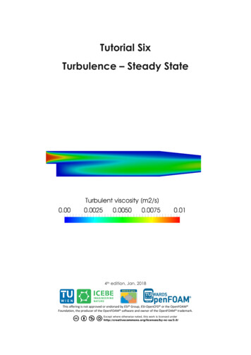
OpenFOAM Basic TrainingTutorial SixsimpleFoam – pitzDailySimulationUse simpleFoam solver, run a steady state simulation with following turbulencemodels: kEpsilon (RAS) kOmega (RAS) LRR (RAS)Objectives Understanding turbulence modeling Understanding steady state simulationData processingShow the results of U and the turbulent viscosity in two separate contour plots.

OpenFOAM Basic TrainingTutorial Six1. Pre-processing1.1. Copy tutorial FOAM TUTORIALS/incompressible/simpleFoam/pitzDaily1.2. 0 directoryWhen a turbulent model is chosen, the value of its constants and its boundary valuesshould be set in the appropriate files. For example in kEpsilon model the k andepsilon files should be edited. See below for the epsilon file:// * * * * * * * * * * * * * * * * * * * * * * * * * * * * * * * * * * * * * * ** * * * * *//dimensions[0 2 -3 0 0 0 0];internalFielduniform form ilonWallFunction;valueuniform form 14.855;}frontAndBack{typeempty;}}// * * * * * * * * * * * * * * * * * * * * * * * * * * * * * * * * * * * * * * ** * * * * *//Note: Here is a list of files which should be available at 0 directory and need to bemodified for each turbulence model: laminar: no file kEpsilon (RAS): k and epsilon kOmega (RAS): k and omega LRR (RAS): k, epsilon and R Smagorinsky (LES): nuSgs kEqn (LES): k and nuSgs – This model is called „oneEqEddy‟ in V2.3.0

OpenFOAM Basic TrainingTutorial Six SpalartAllmaras (LES): nuSgs and nuTildaSome files are available, e.g. epsilon, k and nuTilda, some files should be created bythe user, e.g. R, nuSgs. Templates for these files can be also found in the examples ofolder versions of OpenFOAM , e.g. 1.7.1.Note: A missing R file can be created by OpenFOAM .Open theturbulenceProperties file in the constant directory, set the simulationType to RAS,and RASModel to kEpsilon. Run the command „simpleFoam –postProcess –fun R‟from terminal, it will create the turbulenceProperties:R file in the 0 directory. Thensimply rename the file to „R‟.1.3. constant directoryIn the turbulenceProperties file, the simulationType can be set as either RAS, LESor laminar. Then the corresponding sub-dictionary of the chosen simulation typeneeds to be defined. In this case, the sub-dictionary for RAS contains informationabout the chosen RAS model (kEpsilon), and the status of turbulence andprintCoeffs are turned to on.// * * * * * * * * * * * * * * * * * * * * * * * * * * * * * * * * * * * * * * ** * * * * effskEpsilon;on;on;}// * * * * * * * * * * * * * * * * * * * * * * * * * * * * * * * * * * * * * * ** * * * * *//Note: For the laminar model, set turbulence and printCoeffs to off.1.4. system directoryNote: Since it is a steady state simulation, endTime in controlDict shows the numberof iterations instead of time and deltaT should be 1, because it is the amount ofincrease in the iteration number.For the LRR model, discretization model for the new variable R needs to be specified.It is done through the fvSchemes file,// * * * * * * * * * * * * * * * * * * * * * * * * * * * * * * * * * * * * * * ** * * * * es{steadyState;Gauss linear;

OpenFOAM Basic TrainingTutorial Sixdefaultnone;div(phi,U)bounded Gaussdiv(phi,k)bounded Gaussdiv(phi,epsilon) bounded Gaussdiv(phi,omega)bounded Gaussdiv(phi,v2)bounded Gaussdiv(phi,R)bounded Gaussdiv(R)Gauss tress)GausslinearUpwind gradf(U);limitedLinear 1;limitedLinear 1;limitedLinear 1;limitedLinear 1;limitedLinear 1;Gauss linear;linear;}laplacianSchemes{default}Gauss linear }// * * * * * * * * * * * * * * * * * * * * * * * * * * * * * * * * * * * * * * ** * * * * *//Furthermore, fvSolution needs to be changed due to the new R parameter. The solvertype for R is defined, in this case the solver used will be the same as the one for othervariables (U, k, epsilon, omega).2. Running simulation blockMesh simpleFoamNote: When the solution converges, “SIMPLE solution converged in iterations” message will be displayed in the Shell window. If nothing happens andyou do not see a message after a while (this is not the case in here, it converges aftera short time), then you should check the residuals which are displayed in the Shellwindow manually (you should check initial residual values, it shows thedifference between this iteration and the last one), if all of the Initial residual(see below) values are close to amounts you have set in the fvSolution then you canstop simulation (ctrl c).Time 298smoothSolver: Solving for Ux, Initial residual 0.00013831, Final residual 9.28001e-06, No Iterations 6smoothSolver: Solving for Uy, Initial residual 0.000977894, Final residual 6.73868e-05, No Iterations 6GAMG: Solving for p, Initial residual 0.00192871, Final residual 0.000174838, No Iterations 7time step continuity errors : sum local 0.000840075, global 6.13868e-05,cumulative -0.193739

OpenFOAM Basic TrainingTutorial SixsmoothSolver: Solving for epsilon, Initial residual 0.000175322, Finalresidual 1.138e-05, No Iterations 2smoothSolver: Solving for k, Initial residual 0.000404928, Final residual 2.99083e-05, No Iterations 2ExecutionTime 56.7 s ClockTime 57 sSIMPLE solution converged in 298 iterations3. Post-processingThe simulation results are as follows (all simulations scaled to the same range):RASmodelVelocity magnitudeTurbulent viscositykEpsilonkOmegaLRRVelocity magnitude and turbulent viscosity for different RAS models

Reynolds stress transport models Large eddy simulations Detached eddy simulations and other hybrid models In this tutorial, RANS-based model is explained in detail. In the next tutorial, large eddy simulations (LES) and Smagorinsky-Lilly model will be covered. 2. RANS-based models The governing equations for a Newtonian fluid are: