Transcription
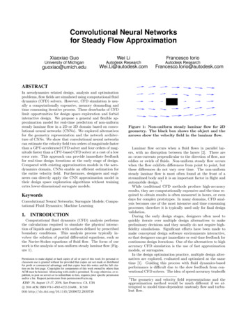
Convolutional Neural Networksfor Steady Flow ApproximationXiaoxiao GuoWei LiFrancesco IorioUniversity of MichiganAutodesk ResearchAutodesk sco.Iorio@autodesk.comABSTRACTIn aerodynamics related design, analysis and optimizationproblems, flow fields are simulated using computational fluiddynamics (CFD) solvers. However, CFD simulation is usually a computationally expensive, memory demanding andtime consuming iterative process. These drawbacks of CFDlimit opportunities for design space exploration and forbidinteractive design. We propose a general and flexible approximation model for real-time prediction of non-uniformsteady laminar flow in a 2D or 3D domain based on convolutional neural networks (CNNs). We explored alternativesfor the geometry representation and the network architecture of CNNs. We show that convolutional neural networkscan estimate the velocity field two orders of magnitude fasterthan a GPU-accelerated CFD solver and four orders of magnitude faster than a CPU-based CFD solver at a cost of a lowerror rate. This approach can provide immediate feedbackfor real-time design iterations at the early stage of design.Compared with existing approximation models in the aerodynamics domain, CNNs enable an efficient estimation forthe entire velocity field. Furthermore, designers and engineers can directly apply the CNN approximation model intheir design space exploration algorithms without trainingextra lower-dimensional surrogate models.KeywordsConvolutional Neural Networks; Surrogate Models; Computational Fluid Dynamics; Machine Learning1.INTRODUCTIONComputational fluid dynamics (CFD) analysis performsthe calculations required to simulate the physical interaction of liquids and gases with surfaces defined by prescribedboundary conditions. This analysis process typically involves the solution of partial differential equations, such asthe Navier-Stokes equations of fluid flow. The focus of ourwork is the analysis of non-uniform steady laminar flow (Figure 1).Permission to make digital or hard copies of all or part of this work for personal orclassroom use is granted without fee provided that copies are not made or distributedfor profit or commercial advantage and that copies bear this notice and the full citation on the first page. Copyrights for components of this work owned by others thanACM must be honored. Abstracting with credit is permitted. To copy otherwise, or republish, to post on servers or to redistribute to lists, requires prior specific permissionand/or a fee. Request permissions from permissions@acm.org.KDD ’16, August 13-17, 2016, San Francisco, CA, USAc 2016 ACM. ISBN 978-1-4503-4232-2/16/08. . . 15.00DOI: http://dx.doi.org/10.1145/2939672.2939738Figure 1: Non-uniform steady laminar flow for 2Dgeometry. The black box shows the object and thearrows show the velocity field in the laminar flow.Laminar flow occurs when a fluid flows in parallel layers, with no disruption between the layers [2]. There areno cross-currents perpendicular to the direction of flow, noreddies or swirls of fluids. Non-uniform steady flow occurswhen the flow exhibits differences from point to point, butthese differences do not vary over time. The non-uniformsteady laminar flow is most often found at the front of astreamlined body and it is an important factor in flight andautomobile design. 1While traditional CFD methods produce high-accuracyresults, they are computationally expensive and the time required to obtain results is often measured in hours, or evendays for complex prototypes. In many domains, CFD analysis becomes one of the most intensive and time consumingprocesses; therefore it is typically used only for final designvalidation.During the early design stages, designers often need toquickly iterate over multiple design alternatives to makepreliminary decisions and they usually do not require highfidelity simulations. Significant efforts have been made tomake conceptual design software environments interactive,so that designers can get immediate or real-time feedback forcontinuous design iterations. One of the alternatives to highaccuracy CFD simulation is the use of fast approximationmodels, or surrogates.In the design optimization practice, multiple design alternatives are explored, evaluated and optimized at the sametime [1]. Guiding this process with fluid dynamics-basedperformance is difficult due to the slow feedback from conventional CFD solvers. The idea of speed-accuracy tradeoffs1The geometry and velocity field representations and theapproximation method would be much different if we attempted to model time-dependent unsteady flow and turbulent flow.
[6] also leads to practical design space exploration and design optimization in the aerodynamics domain by using fastsurrogate models.Data-driven surrogate models become more and more practical and important because many design, analysis and optimization processes generate high volume CFD physical orsimulation data. Over the past years, deep learning approaches (see [5, 26] for survey) have shown great successesin learning representations from data, where features arelearned end-to-end in a compositional hierarchy. This isin contrast to the traditional approach which requires thehand-crafting of features by domain experts. For data thathave strong spatial and/or temporal dependencies, Convolutional Neural Networks (CNNs) [20] have been shown tolearn invariant high-level features that are informative forsupervised tasks.In particular, we propose a general CNN-based approximation model for predicting the velocity field in 2D or 3Dnon-uniform steady laminar flow. We show that CNN basedsurrogate models can estimate the velocity field two ordersof magnitude faster than a GPU-accelerated CFD solveror four orders of magnitude faster than a CPU-based CFDsolver at a cost of a low error rate. Another benefit of usinga CNN-based surrogate model is that we can collect trainingdata from either physical or simulation results. The knowledge of fluid dynamics behavior can then be extracted fromdata sets generated by different CFD solvers, using differentsolution methods. Traditional high accuracy simulation isstill an important step to validate the final design, but fastCFD approximation models have wide applications in theconceptual design and the design optimization process.2.2.1RELATED WORKCFD AnalysisComputational methods have emerged as powerful techniques for exploring physical and chemical phenomena andfor solving real engineering problems. In traditional CFDmethods, Navier-Stokes equations solve mass, momentumand energy conservation equations on discrete nodes (thefinite difference method, FDM) [11], elements (the finite element method, FEM) [29], or volumes (the finite volumemethod, FVM) [24]. In other words, the nonlinear partialdifferential equations are converted into a set of non-linearalgebraic equations, which are solved iteratively. TraditionalCFD simulation suffers from long response time, predominantly because of the complexity of the underlying physicsand the historical focus on accuracy.The Lattice Boltzmann Method (LBM) [22] was introduced to overcome the drawbacks of the lattice gas cellularautomata. In LBM, the fluid is replaced by fractious particles. These particles stream along given directions (latticelinks) and collide at the lattice sites. LBM can be considered as an explicit physical-based approximation method.The collision and streaming processes are local [23]. LBMemerged as an alternative powerful method for solving fluiddynamics problems, due to its ability to operate with complex geometry shapes and to its trivially parallel implementation nature [31, 21]. Since distinct particle motion canbe decomposed over many processor cores or other hardware units, efficient implementations on parallel computersare relatively easy. LBM can also handle complex boundaryconditions. However, LBM still requires numerous iterationsand its convergence speed depends on the geometry boundaries. In this paper, we use LBM to generate all the trainingdata for the CNNs, and we compare the speed of our CNNbased surrogate models with both traditional CPU LBMsolvers and GPU-accelerated LBM solvers.Compared with physical-based simulation and approximation methods, our approach falls into the category of datadriven surrogate models (or supervised learning in machinelearning). The knowledge of fluid dynamics behavior can beextracted from large data sets of simulation data by learningthe relationship between an input feature vector extractedfrom geometry and the ground truth data output from a fullCFD simulation. Then, without the computationally expensive iterations that a CFD solver requires to allow the flowto converge to its steady state, we can directly predict thesteady flow behavior in a fraction of the time. The number ofiterations and runtime in a CFD solver is usually dependenton the complexity of geometries and boundary conditions,but they are irrelevant to those factors in the predictionprocess. Note that only the prediction runtime of surrogatemodels has a significant impact on the design processes. Thetraining time of the surrogate models is irrelevant.2.2Surrogate Modeling in CFD-based DesignOptimizationThe role of design optimization has been rapidly increasing and evolving in aerodynamics related fields, such asaerospace and architecture design [1]. CFD solvers havebeen widely used in design optimization (finding the bestdesign parameters that satisfy project requirements) and design space exploration (finding multiple designs that satisfythe requirements). However, the direct application of a CFDsolver in design optimization is usually computationally expensive, memory demanding and time consuming. The basic idea of using surrogates (approximation models) is toreplace a high-accuracy, expensive analysis process with aless expensive approximation. CFD surrogate models can beconstructed from physical experiments [30]. However, highfidelity numerical simulation proves to be reliable, flexible,and relatively cheap compared with physical experiments(see [1] and references therein).Various surrogate models have been explored for designprocesses, such as polynomial regression [12, 3], multipleadaptive regression splines (MARS) [10], Kriging [12, 16],radial basis function network [19], and artificial neural networks [7, 4]. The existing approaches only predict a restricted subset of the whole CFD velocity field. For example, predict the pressure on a set of points on an object surface [32]. Most existing approaches also depend ondomain-specific geometry representations and can only beapplied to low-order nonlinear problems or small scale applications [10, 18]. The models are usually constructed bymodeling the response of a simulator on a limited numberof intelligently chosen data points. Instead of modeling eachindividual low-dimensional design problem, we model thegeneral non-uniform steady laminar CFD analysis solution,so that our model can be reused in multiple different, lowerdimensional optimization processes, and predict the wholevelocity field.2.3Convolutional Neural NetworksConvolutional neural networks have been proven successful in learning geometry representations [27, 13]. CNNs
also enable per-pixel predictions in images. For example,FlowNet [8] predicts the optical flow field from a pair of images. Eigen, Puhrsch and Fergus [9] estimate depth from asingle image. Recently, CNNs are applied on voxel to voxelprediction problems, such as video coloring [28].Our approach applies CNNs to model large-scale nonlinear general CFD analysis for a restricted class of flowconditions. Our method obtains a surrogate model of thegeneral high-dimensional CFD analysis of arbitrary geometry immersed in a flow for a class of flow conditions, andnot a model based on predetermined low-dimensional inputs.For this reason, our model subsumes a multitude of lowerdimensional models, as it only requires training once and canbe interrogated by mapping lower-dimensional problems intoits high-dimensional input space. The main contribution ofour CNN based CFD prediction is to achieve up to two tofour orders of magnitude speedup compared to traditionalLattice Boltzmann Method (LBM) for CFD analysis at acost of low error rates.3.CONVOLUTIONAL NEURAL NETWORKSURROGATE MODELS FOR CFDWe propose a computational fluid dynamics surrogate modelbased on deep convolutional neural networks (CNNs). CNNshave been proven successful in geometry representation learning and per-pixel prediction in images. The other motivationof adopting CNNs is its memory efficiency. Memory requirement is a bottleneck to build whole velocity field surrogatemodels for large geometry shapes. The sparse connectivity and weight-sharing property of CNNs reduce the GPUmemory cost greatly.Our surrogate models have three key components. First,we adopt signed distance functions as a flexible and generalgeometric representation for convolutional neural networks.Second, we use multiple convolutional encoding layers to extract abstract and high-level geometric representations. Finally, there are multiple convolutional decoding layers thatmap the abstract geometric representations into the computational fluid dynamics velocity field.In the rest of this section, we describe the key componentsin turn.3.1Figure 2: A discrete SDF representation of a circle shape (zero level set) in a 23x14 Cartesian grid.The circle is shown in white. The magnitude of theSDF values on the Cartesian grid equals the minimaldistance to the circle.A signed distance function D(i, j) associated to a level setfunction f (i, j) is defined byD(i, j) min(i0 ,j 0 ) Z(i, j) (i0 , j 0 ) sign(f (i, j))(2)D(i, j) is an oriented distance function and it measures thedistance of a given point (i, j) from the nearest boundary ofa closed geometrical shape Z, with the sign determined bywhether (i,j) is inside or outside the shape. Also, every pointoutside of the boundary has a value equal to its distance fromthe interface (see Figure 2 for a 2D SDF example).Similarly, given a discrete representation of a 3D geometryon a Cartesian grid, the signed distance function isD(i, j, k) min(i0 ,j 0 ,k0 ) Z(i, j, k) (i0 , j 0 , k0 ) sign(f (i, j, k))(3)A demonstration of 3D SDF is shown in Figure 3, whereSDF equals to zero on the cube surface. In this paper, weuse the Gudonov Method [14, 25] to compute the signeddistance functions.Geometry RepresentationGeometry can be represented in multiple ways, such asboundaries and geometric parameters. However, those representations are not effective for neural networks since thevectors’ semantic meaning varies. In this paper, we use aSigned Distance Function (SDF) sampled on a Cartesiangrid as the geometry representation. SDF provides a universal representation for different geometry shapes and worksefficiently with neural networks.Given a discrete representation of a 2D geometry on aCartesian grid, in order to compute the signed distance function, we first create the zero level set, which is a set of points(i, j) that give the geometry boundary (surface) in a domainΩ R2 : Z (i, j) R2 : f (i, j) 0(1)where f is the level set function s.t. f (i, j) 0 if and onlyif (i, j) is on the geometry boundary, f (i, j) 0 if and onlyif (i, j) is inside the geometry and f (i, j) 0 if and only if(i, j) is outside the geometry.Figure 3: Signed distance function for a cube in 3DdomainThe values of SDF on the sampled Cartesian grid not onlyprovide local geometry details, but also contain additional
information of the global geometry structure. To validatethe efforts of computing SDF values in our experiments, wecompare the geometry representiveness of SDF and a simplebinary representation, where a grid value is 1 if and only ifit is within or on the boundary of geometry shapes. Suchbinary representations are easier to compute, but the valuesdo not provide any global structure information. We empirically show that SDF is more effective in representing thegeometry shapes for convolutional neural networks.3.22D convolution decoding3D convolution decoding2D convolution encoding3D convolution encodingFigure 5: Convolution encoding and decoding.CFD SimulationIn this paper, we intend to leverage deep neural networksas real-time surrogate models to substitute traditional timeconsuming Lattice Boltzmann Method (LBM) CFD simulation [22]. LBM represents velocity fields as regular Cartesiangrids, or lattices, where each lattice cell represents the velocity field at that location. The LBM procedure updatesthe lattice iteratively, and usually the amount of requirediterations for the flow field to stabilize from a cold start islarge.In LBM, geometry is represented by assigning an identifierto each lattice cell. This specific identifier defines whethera cell lies on the boundary or in the fluid domain. Figure 4 illustrates this using an example of a 2D cylinder ina channel. In general, the LBM lattice cell resolution doesnot necessarily equal to the SDF resolution. In this work,we use the same geometry resolution in the LBM simulationand in the SDF representation. Thus, for a geometry withH W D SDF representation, its CFD velocity field isalso H W D. A 2D velocity field consists of two components x and y to represent the velocity components inx-direction and y-direction respectively. The velocity fieldfor 3D geometry has one additional z-component to represent the velocity component in the z-direction.encoded feature vector henc (s) can be formulated as:henc (s) ConvNN(s)(4)where ConvNN(.) denotes the mapping from the SDF to ageometry representation vector using multiple convolutionlayers and a fully connected layer at the end, each of whichis followed by a rectifier non-linearity (ReLU).3.4Convolutional DecodingWe use the ’inverse’ operation of convolution, called deconvolution, to construct multiple stacked decoding layers.Deconvolution layers multiply each input value by a filterelementwise, and sum over the resulting output windows.In other words, a deconvolution layer is a convolution layerwith the forward and backward passes reversed. 2D deconvolution maps 1 1 spatial region of the input to w hconvolution kernels. 3D deconvolution maps 1 1 1 spatial region of the input to w h d convolution kernels, asshown in Figure 5.In our method, deconvolution operations are used to decode high-level features encoded and transformed by the encoding layers. The decoding procedure can be representedas:t̂x (s) DeconvNN(henc (s))(5)xwhere t̂ (s) denotes the x-component prediction of the CFDvelocity field. DeconvNN(.) is a mapping from the extractedgeometry representation vector to CFD velocity field component using multiple deconvolution layers, each of whichis followed by a rectifier non-linearity (ReLU). We decodethe y-component (and z-component for 3D geometry) of theCFD velocity field in the same way.3.5Network Architecture andEnd-To-End TrainingEuclideanLossFigure 4: 2D channel flow definition for LBM(1 fluid, 2 no-slip boundary, 3 velocity boundary,4 constant pressure boundary, 5 object boundary,0 internal)ith componentsof CFDconvolution encodingconvolution decodingith outputjth componentsof CFDSDF3.3Convolution EncodingThe encoding part takes the SDF, s, as an input, andstacked convolution layers extract geometry features directlyfrom the SDF representation. For 2D geometry, s is a matrixthat sij D(i, j) and the 2D convolution operations areused for encoding. For 3D geometry, s is a 3D tensor thatsijk D(i, j, k), and the encoding uses 3D convolution. Thejth outputFigure 6: CNN based CFD surrogate model architectureWe use a shared-encoding and separated-decoding architecture for our CFD surrogate model in Figure 6. The
shared-encoding saves computations compared to separatedencoding alternatives. Unlike encoding layers, decoding layers are interfered by different velocity field components whena shared-decoding structure is used. In our shared-encodingand separated-decoding architecture, multiple convolutionallayers are used to extract an abstract geometry representation, and the abstract geometry representation is used bymultiple decoding parts to generate the various componentsof the CFD velocity field. There are two decoding parts for2D geometry shapes and three for 3D geometry shapes. Analternative encoding structure is to use separated encodinglayers for each decoding part. In the experiment section, weshow that the prediction accuracy of the separated encodingstructure is similar to the shared encoding structure.Further, we condition our CFD prediction based on theSDF to reduce errors. By definition, the velocity inside andon the boundary of geometry shapes is zero. Thus, the velocity field values change dramatically on the boundary ofgeometry shapes. SDF itself fully represents the boundaryinformation and our neural networks could condition theprediction by masking out the pixel or voxel inside or onthe boundary of the geometry. Such conditioned prediction eases the training and improve the prediction accuracy.The final prediction of our model is tˆx 1{s 0}, where1{s 0} is a binary mask and has the same size as s. Itselement is 1 if and only if the corresponding signed distancefunction value is greater than 0. denotes element-wiseproduct.We train our model to minimize the mean squared error:L(θ) N1 X ˆx t (sn ) 1{sn 0} tx (sn ) 2N n 1(6) tˆy (sn ) 1{sn 0} ty (sn ) 2A similar loss function is defined for 3D geometry shapes:L(θ) N1 X ˆx t (sn ) 1{sn 0} tx (sn ) 2N n 1 tˆy (sn ) 1{sn 0} ty (sn ) 2(7) tˆz (sn ) 1{sn 0} tz (sn ) 24.EXPERIMENT SETUPIn the experiments, we evaluate our proposed method inboth 2D and 3D geometry domains. In the 2D domain, wetrain the convolutional neural networks using a collectionof 2D geometric primitives and evaluate the prediction overa validation dataset of 2D primitives and a test dataset of2D car shapes (see Figure 7 for examples). We then train aseparate network using a collection of 3D geometry shapesinside a channel (see Figure 8 for examples) and evaluate theprediction over a validation dataset of 3D geometry shapes.We first empirically compare the representiveness of SDFwith the simple binary representations and show that SDFoutperforms binary representations in CFD prediction. Second, our CNN based surrogate model outperforms a patchbased linear regression baseline in predicting CFD for both2D and 3D geometry shapes. Finally, we compare the timecost of our proposed method with traditional LBM solversto highlight the speedup of our proposed method.We begin by describing the details of the datasets, LBMdata generation, convolutional neural network architectures,and training parameters.4.1Data and PreprocessingFigure 7: 2D car dataset visualization.Figure 8: 3D channel dataset: two 3D primitives (arectangular box and a sphere) in a 32-by-32-by-32channel and the visualization of their SDF on theY-Z plane2D data set. The 2D training and validation datasets consist of 5 types of simple parametric geometric 2D primitives: triangles, quadrilaterals, pentagons, hexagons and dodecagons. Each set of primitives contains samples that aredifferent in size, shape, orientation and location. The training dataset contains 100,000 samples (20,000 random samples for each kind of primitives), and the validation datasetcontains 10,000 samples (2,000 random samples for each kindof primitives). The 2D primitives are projected into a 256by-128 Cartesian grid and the LBM simulation computes a256-by-128 velocity field as labels. We construct two kindsof 2D primitive datasets for different boundary conditions.In Type I, the primitives are always connected to the lowerboundary. In Type II, the primitives are always above thelower boundary, and the gap ranges from 15 to 25 pixels.2D car test data set. This data set is dedicated to testthe generalization ability of our trained models. It containsvarious kinds of car prototypes, such as jeeps, vans and sportcars. The car samples are not visible in the training. Similarto 2D primitives, the car samples are projected into a 256by-128 Cartesian grid and the LBM simulation computesa 256-by-128 velocity field. We also create two boundaryconditions for the car samples.3D data set. In order to understand whether interactionsof flow with sets of multiple boundaries can be learned effectively, the 3D dataset contains 0.4 million sphere and rectangular prism pairs. Each sphere-prism pair is positioned ina 32 32 32 channel. Both the location and the parametersof each 3D object are randomly generated. Then a LBMsimulation is performed on the 3D channel, where the fluidenters the channel along the x axile.
SDF preprocessing. We performed pixel/voxel-wise meanremoval for SDF and scaled the resulting representation by0.01 as inputs to the CNNs.4.2Network Architectures and TrainingThe architectures and hyper-parameters of our CNN surrogate models for 2D and 3D CFD are shown in Figure 9.In the CNN architectures, the encoding part is shared bydecoding parts for different CFD dimensions. Alternativearchitectures could use a separated encoding part for eachdecoding part where each separated encoding part has thesame architecture and hyper-parameters as the shared encoding part. We compare these two encoding paradigms inour experiments.We implemented the CNNs using Caffe [17]. The parameters of the networks were initialized using Xavier method inCaffe. We used RMSProp with a batch size of 64 to optimizethe parameters of the convolutional neural networks. TheRMS decay parameter was set to 0.05. We set the initiallearning rate to be 10 4 and multiplied the learning rate by0.8 for every 2500 iterations.5.err CFD Solver ConfigurationLaminar flow occurs at low Reynolds numbers2 , whereviscous forces are dominant, and is characterized by a fluidflowing in parallel layers, with no disruption between thelayers. In all the experiments, we used a Reynolds numberof 20. For our 2D experiments, we used OpenLB [15], a C Lattice Boltzmann library, to generate CFD velocity field.Because of the lack of GPU support in OpenLB, we raneach simulation on a single core on a Intel Xeon E5-2640V2processor. For our 3D experiments, we used a proprietaryGPU-accelerated LBM solver.4.3The average relative error over the test data set is themean of all the test cases:EXPERIMENT RESULTSWe use the average relative error [1] in the CFD literatureto evaluate our prediction. We first compute the differencebetween the predicted velocity field and the LBM generatedvelocity field. For a pixel/voxel, the relative error is definedas the ratio of the magnitude of the difference to the LBMgenerated velocity field. For 2D geometry shapes, the relative error at pixel (i, j) in n-th test case is represented as:q(tˆxij (sn ) txij (sn ))2 (tˆyij (sn ) tyij (sn ))2qerrn (i, j) txij (sn )2 tyij (sn )2(8)The average relative error of n-th data case is the mean valueof all the pixels outside the geometry shape:P Perrn (i, j)1ij (sn 0)iPj P(9)errn ij 1ij (sn 0)where 1ij (sn 0) is 1 if and only if (i, j) is outside ofthe geometry boundary of sn . errn can be extended to3D geometry shapes straightforwardly by considering thez-component.2In CFD modeling, the Reynolds number is defined as a nondimensional ratio of the inertial forces to viscous forces andquantifies their relevance for the prescribed flow condition[2].5.1N1 X nerrN n 1(10)Signed Distance Function vs. Binary RepresentationOne contribution of this paper is proposing using SDF asgeometric representations for the CNN models. We evaluatethe effectiveness of SDF geometric representations by comparing with the binary representations in the same CNN architectures. In the experiments, the binary representationsuse a 256 128 binary matrix to represent the geometry.Its element is 1 if and only if the corresponding position ison the geometry boundary or inside the geometry.The results of prediction on 2D primitives are summarizedin the Table 1.DataSet2D Type I2D Type IIEncoding 6%3.08%Binary54.60%55.25%74.52%80.71%Table 1: 2D CFD prediction results of SDF and binary representations.The results show that the errors of using SDF are significantly smaller than the errors of using binary representations. Given that the deep neural networks are the same,the results imply that the SDF representations are more effective than the binary representations. Each value in theSDF representations carries a certain level global information while the values in binary representations only carryrestricted local information. Due to such difference, binaryrepresentations may require more complex architectures tocapture whole geometric information properly. We also compare the SDF representations to the first order gradients ofthe SDF representations, the prediction accuracy improvement is not significant, so we focus our contributions on using SDF because of its computation simplicity. The resultsalso show that the prediction accuracy of shared encoding issimilar to that of separated encoding.5.2Patch-wise Linear Regression BaselineA patch-wise linear regression model is applied as a baseline to evaluate our proposed models. For 2D geometryshapes, the 256 128 SDF inputs are divided into 32 32 patches without overlap. The patch-wise linear regression model takes 32 32 patches as inputs and predicts 32 32 patches to construct the CFD velocity field for eachcomponent. The predicted 32 32 patches are concatenatedwithout overlap to form the x-component or y-component ofthe CFD velocity field. For 3D geometry shapes, the 32 32 32 SDF inputs are divided into 8 8 8 patcheswithout overlap, and the predicted 8 8 8 patches arethen concatenated to form the velocity field.The prediction results of CNNs and baseline are summari
CFD simulation. Then, without the computationally expen-sive iterations that a CFD solver requires to allow the ow to converge to its steady state, we can directly predict the steady ow behavior in a fraction of the time. The number of iterations and runtime in a CFD solver is usually dependent on the complexity of geometries and boundary .