Transcription
Single-Family Client and Community Engagement NoteAUGUST 2022Freddie Mac First-Time HomebuyerAffordability Map: A Novel Approach toMeasure Affordability for Future BorrowersFirst-time homebuyers play a critical role in sustaining the housing ecosystem.Unlike repeat homebuyers who have more robust credit history, first-time homebuyersmay not qualify for the best mortgage rates in the market. Moreover, they tend to beyounger and hence have lower income and savings, which further fuels the challengeof housing affordability. In this research, we build a new methodology to evaluatethe local affordability for future first-time homebuyers. Our unique approach enablesus to calibrate the affordability measure by race and various income groups,through which we uncover some unexpected patterns.IntroductionFirst-time homebuyers play a critical role in sustaining the housing ecosystem. According to Bai, Zhuand Goodman (2015), they allow current homeowners to sell and move to a new town, a new job,a retirement community, or upgrade to a bigger house. Even during the pandemic, the share of first-timehomebuyers remained strong at 31% according to the National Association of Realtors (NAR). As theeconomy slowly recovers from the pandemic, affordability for future first-time homebuyers is ambiguous.While mortgage interest rates remained historically low during the pandemic, they’re quickly climbingand other factors such as a weak labor market, higher house prices, very low inventory and studentloan debt obligations, will make it challenging for future borrowers to transition into homeownership.While the fiscal stimulus aid may have mitigated the impact of the financial shock on future borrowerssomewhat, it is still relatively difficult for borrowers without high credit to obtain conventionalmortgages.1 Furthermore, as the nation is recovering, the speed of recovery will vary across localities,making local affordability for future first-time homebuyers even more uncertain.1Mortgage Credit Availability Map published by Mortgage Bankers Association declined significantly since March 2020 which is indicative of tighteninglending standards. See availabilityindex-x241340. Also see g-mortgage-credit-box. 2022 Freddie Macwww.freddiemac.com
In this research, we propose a new methodology to evaluate the local affordability for future borrowersbased on their credit characteristics and income distribution. The Freddie Mac First-Time HomebuyerAffordability Map (FFTHAM) was developed using uniquely constructed anonymized administrativedatasets that measure how many creditworthy renters have enough income to purchase a home thatwas bought by a recent first-time homebuyer with a comparable credit profile in the area. In addition,our map allows us to specifically investigate the local affordability by race and various income groups.For example, we can examine the local affordability for the low- to moderate-income (LMI) creditworthypopulation who are generally more challenged to find affordable housing options in their areas.2 Lastly,our map measures affordability over the last decade (i.e., 2012-2020) and allows us to track the extent towhich economic shocks, such as the current pandemic, have impacted the local affordability for futureborrowers, especially for low income and minority families.Our FFTHAM rank orders cities into four different affordability categories by income: 1) typicallyaffordable, such as Knoxville, TN, 2) typically unaffordable, such as San Francisco, CA, 3) affordableoverall but not affordable to its LMI population, and 4) unaffordable overall but affordable to its LMIpopulation. In particular, we found that there could be material gaps between the affordability for LMIpopulations and overall population in some areas. For example, certain southern metropolitan statisticalareas (MSAs), such as El Paso, TX, that appear overall affordable are unaffordable to their LMI population,predominantly due to their low area median income, making it very challenging for LMI families toafford a home in these cities. In contrast, certain coastal cities such as Baltimore, MD that appear to beoverall unaffordable, are affordable to their LMI families, likely due to the availability of many relativelyaffordable housing options in the area.Our FFTHAM by race/ethnicity shows that, for a given metroarea, creditworthy renters who are White are more likely to havehigher affordability than their counterparts who are HispanicAmericans or Black Americans. Furthermore, affordability hasdeclined over time for most future borrowers regardless of race/ethnicity. In particular, Hispanic Americans living in high-costcoastal cities have experienced a sharp decline in affordabilitysince 2012. Lastly, the pandemic crisis triggered a decline inaffordability in most cities, likely due to a surge in demand andlack of inventory.The pandemic crisis triggered adecline in affordability in mostcities, likely due to a surge indemand and lack of inventory.A variety of indexes exist to help us better understand the affordability challenges in the country.3Common industry level affordability metrics focus on median income and median house prices and arebased on the entire population, which includes both renters and homeowners. Very few affordabilityindexes focus on low-income households. Several authors have pointed out that affordability is a biggerconcern in the lower end of the income distribution (Gan and Hill, 2009; Jewkes and Delgadillo, 2010).Quigley and Raphael (2004) show that there is little evidence supporting that housing has become lessaffordable to a median homeowner or renter in recent years. However, there has been a pronouncedincrease in the rent burden of low and very-low-income households, adding more constraints to theirhomeownership potential. Urban Institute’s Housing Affordability for Renters Index (HARI) address someof these shortcomings by considering the entire income distribution rather than the median household.Furthermore, the Urban Institute index evaluates the potential of only the renter population to becomefirst-time homebuyers, which is more forward looking than existing indices.23Low- to moderate-income population refers to those who made 80% or less area median income.See Linneman and Megbolugbe, 1992; Bogdan and Can, 1997; Fannie Mae 2015; Haurin 2016; Jewkes and Delgadillo, 2010.Single-Family Client and Community Engagement Note August 20222
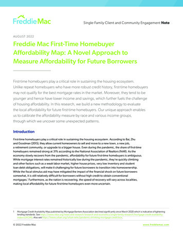
Our FFTHAM builds upon existing industry statistics and compares the entire income distribution ofrecent first-time homebuyer and creditworthy renter populations in assessing who can afford a house.To be precise, our map offers improvement on existing methodologies in three ways. First, our uniquedataset obtained from a credit bureau allows us to account for credit scores and simple underwritingstandards to identify “Mortgage Ready” or creditworthy renters.4 Renters’ creditworthiness not onlyimpacts their ability to secure a mortgage, but also to make their monthly payments (Fannie Mae, 2015).By purging the renters with lower credit scores, higher debt-to-income ratios, and derogatory credithistories, we are able to align our renter population more closely with future borrowers as opposed toHARI, which includes all renters as potential first-time homebuyers. Moreover, our map allows usto investigate how affordability for creditworthy renters varies by various minority and/or incomegroups and over time.Second, we assess home affordability for current renters based on only those consumers that haverecently purchased their first home as a primary residence, unlike HARI, which is based on all recenthomeowners. According to Bai, Zhu and Goodman (2015), an average first-time homebuyer is morelikely to have smaller loan size, lower credit scores, higher loan-to-value and debt-to-income ratios,thus obtaining higher interest ratescompared to an average repeat buyer.EXHIBIT 1:This implies we may overestimateShare of First-Time Homebuyer between 2010-2020the affordability of homes for futureborrowers based on recent activities58.7%by repeat purchasers. We assume57.4%first-time home purchasers, whogenerally have less experience in themortgage process relative to repeat54.7%borrowers, better represent the54.1%54.0%future borrowers. Using loan-level53.0%data from the National Mortgage52.0%51.9%51.6%51.6%Database (NMDB), we define first51.2%time homebuyers as borrowers whohave not a had a mortgage in thepreceding seven years (see ConsumerFinancial Protection Bureau report).Exhibit 1 gives the share of homepurchase loans originated for firsttime homebuyers each year 010. First-time homebuyers compriseSource: National Mortgage Database (NMDB) 12.1 data from 2010 to 2020, based on credit records ofmore than 50% of the purchaseOctober 14th, 2020.market coming out of the financialNote: Loans are first-lien, owner-occupied originations for home purchase. First Time Home Buyer definedcrisis and are crucial for driving futureby not having a previous mortgage in the credit record, which can go back up to 7 years.homeownership rates.5 By preciselyestimating this sub-group, we are45Our approach to define “Mortgage Ready” consumers is a research-based criterion and not underwriting criterion. While there may be an overlap,we do not know how many “Mortgage Ready” renters will go through underwriting or consider underwriting. For details, see 21-future-borrowers.Our estimates of first-time homebuyer share differ from NAR’s estimate of around 31% in 2020. There are two main reasons for this discrepancy. First, whileour measure is based on loan-level administrative data, NAR’s measure is based on survey results. Second, while our loans are limited to first-lien, owneroccupied originations for home purchase, NAR’s survey includes owner-occupied homes, investor properties, vacation homes and all-cash purchases.Single-Family Client and Community Engagement Note August 20223
able to make an apples-to-apples comparison of homeownership potential of future borrowers.It can also serve as leading indicator of local trends in homeownership rate. To our knowledge,we are the first to develop a forward-looking affordability measure for creditworthy renters basedon information of recent first-time homebuyers. Our map can serve as a leading indicator of futurehomeownership rates by various localities.Lastly, unlike most indexes and tools, our focus is on evaluating the local affordability by various subpopulations. We calibrate the affordability map of renters based on their income relative to the areamedian income to compare the affordability of LMI across cities. An area that appears to be overallaffordable may not be affordable to its LMI population, especially if it is a high-cost area with a lowArea Median Income (AMI). Local affordability can serve as indicators for future homeownership andforeclosures. Wang and Immergluck (2019) investigate the relationship between location affordability,a measure of housing and transportation affordability combined, and foreclosure resilience acrossmetropolitan areas post-financial crisis. They find foreclosure rates dropped substantially in high-densityareas where location affordability is high, but not in low-density areas.The rest of the report is organized as follows: Section 2 reviews the literature on various affordabilityindexes used by the industry, government, and advocates; Section 3 describes the data andmethodology; Section 4 discusses the affordability map and how it is trending over time; Section 5 plotsthe trends in affordability for various sub-groups, section 6 discusses the relationship of the map withhomeownership rate; and Section 7 concludes the report.Literature reviewMost of the housing affordability map metrics are constructed by comparing the amount a householdcan afford for housing to the cost of housing. If the affordable amount is bigger than the cost, then itindicates affordability.One of the most widely used approaches is the ratio approach. It is based on the idea that if a householdpays more for housing than a certain percentage of its income, then it will not have enough to meetfor other non-housing needs. In the definitional terminology used by the United States Department ofHousing and Urban Development (HUD) if total annual housing costs, including principal and interestpayments on the mortgage, property taxes, utilities and insurance, exceed 30% of gross annual income,then the household is “housing cost burdened.” HUD’s measure is widely used as a legislative andregulatory standard to qualify applicants for housing assistance, such as allocation of low-income taxcredits and housing vouchers. The National Low-Income Housing Coalition uses information from HUDto develop Housing Wage that estimates a worker’s ability to afford the Fair Market Rent in a givenarea (Pelletiere, 2008). Despite that, HUD’s measure is criticized as it fails to take into considerationcost-of-living variables or control for quality of housing over time (Bogdon & Can, 1997; Linneman &Megbolugbe, 1992, Pelletiere, 2010, Jewkes and Delgadillo, 2010).Other popular industry measures of affordability are as follows. NAR’s Housing Affordability Index isan indicator of housing affordability that measures whether or not a typical family could qualify for amortgage loan on a typical home, under the assumption of 20% down payment and that the monthlyprincipal and interest payment on the mortgage does not exceed 25% of the median family monthlyincome (Linneman & Megbolugbe, 1992). The National Association of Home Builders (NAHB)/WellsFargo Home Opportunity Index and the California Association of Realtors (CAR) Housing AffordabilityIndex are based on the share of available affordable housing stock for typical families. They assume 28%and 30 percent, respectively, of gross area median income as the affordable amount for a typical familySingle-Family Client and Community Engagement Note August 20224
and consider property taxes and property insurance for a home in a given area along with the mortgagepayment. Bourassa and Haurin (2016) improvised on NAR and NAHB indexes by developing an indexthat includes income tax deductions for mortgage interest and property taxes as well as accounts forthe effect of expected house price changes on affordability of housing. Recently, the Federal HousingFinance Agency developed its affordability index, which estimates a unique affordable ratio for eachMSA by extracting expenditure from income using detailed data sources (see Chung et al, 2018).They consider debt and funds available for down payment, as well as future growth in income, houseprice and expenses.6Both NAR and CAR affordability indexes have variants focusing on affordability of first-time homebuyers.In particular, NAR’s First-Time Homebuyer Index, HAI, is a scaled-down version of its general HAI, sinceit is based on 85% of median house prices, 65% of median income, 10% down payment andcorresponding primary mortgage insurance premium.7 By contrast, CAR’s First-Time Homebuyer HAIassumes adjustable mortgage rates with accompanying points and fees and qualifying income ratio at40%. Related to these, Goldman Sachs developed a methodology to assess the affordability of “marginalborrowers,” who lack the incomes and credit scores to qualify for low mortgage rates.8A second approach of measuring housing affordability is theresidual income approach, which is based on the idea thathouseholds have affordability issues if they cannot meet aThe residual income approachthreshold of non-housing consumption after covering theiris based on the idea thathousing costs. These thresholds vary by level of income,household size and household types. Stone (1990, 1993, 2006)households have affordabilityintroduced the term “Shelter Poverty” as occurring whenissues if they cannot meethousing costs are so high that households cannot afford nona threshold of non-housinghousing necessities under the Bureau of Labor Statistics lowbudget standards. Kutty (2005) introduces “housing-inducedconsumption after coveringpoverty,” which is based on the minimum of non-housingtheir housing costs.consumption at two-third of the U.S. Census Bureau’s povertythreshold.9 The VA home loan program uses residual incomeas a credit underwriting factor to determine the cost burdenon potential borrowers (see VA Pamphlet 26-7).10 Herbert,Hermann and McCue (2018) show that while the residual income approach yields comparable resultsto simple measures like HUD’s 30% of income standard for overall levels of affordability, it does a betterjob in gauging housing affordability challenges for high-cost markets and for higher-income and smallerhouseholds.A third approach involves amenity-based affordability indexes, which incorporate certain location-basedamenities in housing cost estimates. Fisher, Pollakowski and Zabel (2009) adjust their affordability indexto account for town-specific amenities such as job accessibility, school quality and safety. They use ahedonic price equation to estimate implicit prices of these amenities. Their index focuses on the new6FHFA’s tool offers improvement from NAR, NAHB and CAR tools as it incorporates real contemporary and historical data on income, debt and fundsavailable for down payments. It also allows to evaluate affordability at different income distributions other than the median income.7 See otes/pdf/housing-insights-111215.pdf.8 See as-it-looks/.9 While Kutty’s method uses pre-tax income measures to compute nonshelter costs, Stone’s method uses after-tax income. Further, Kutty’s choice ofnonshelter standard based on federal poverty threshold is lower than BLS lower-budget standard used by Stone.10 Residual income is calculated as the amount of net income remaining after deductions of debts and obligations and monthly shelter expenses to coverfamily living expenses such as food, health care, clothing and gasoline.Single-Family Client and Community Engagement Note August 20225
entrants to the market, specifically households earning 50% or more of AMI.11 HUD and Department ofTransportation’s Location Affordability Index uses a statistical modeling framework that considers otherfactors, such as car and transit usage, as potentially related to things that may drive affordability as wellas important determinants of affordability at the census tract level.12Lastly, the Urban Institute’s Housing Affordability for Renters Index (HARI) is based on income distributionand has fewer assumptions than approaches discussed above (Goodman, Li, and Zhu 2018). It does notassume or estimate the percentage of the income that can be spent on housing. It also does not usethe area median income and median house price to calculate the affordable income and housing cost.Instead, it measures how many renters have enough income to purchase a home by comparing renters’income distribution to recent borrowers’ income distribution. If a renter has income greater than or equalto the income earned by households who recently purchased a home using a mortgage, then this rentercan afford a house in the area. Using this methodology, HARI can be constructed at various geographiclevels to understand how affordable an area is for renters already living in the area compared to rentersoutside the area (Goodman and Zhu, 2019, 2020).Data and methodologyTo identify creditworthy renters, we use a uniquely constructedconsumer credit dataset that combines anonymized individualcredit bureau records with credit bureau’s marketing data for theperiod of 2012-2020. The core credit bureau data—onto whichthe anonymized marketing data are merged—spans throughthe entire universe of credit visible population in the UnitedStates present in each archive. The dataset contains detaileddebt and credit information, as well as a wealth of demographicinformation, such as race and ethnicity, age, gender, andgeographic location. Please see Appendix A for more details.We define “Mortgage Ready”as potential future borrowerswho do not currently own amortgage but have observablecredit attributes that may allowthem to qualify for a mortgage.Using this dataset, we define future borrowers or “MortgageReady” as those who do not currently own a mortgage buthave observable credit attributes that may allow them to qualifyfor a mortgage.13 For example, a “Mortgage Ready” renter should meet the following criteria: age 45and below and currently have no mortgages, have a credit score of 660 or higher, a debt-to-incomeratio of 25% or less, no bankruptcies or foreclosures, and no severe delinquencies in the last 12 months(see Freddie Mac report, 2021). Renters tend to have lower credit scores than the overall borrowers onaverage. However, “Mortgage Ready” renters are more likely to have credit profiles similar to the recentfirst-time homebuyers. Thus, “Mortgage Ready” population can better represent future borrowers.11 After accounting for local amenities, their tool reveals major shifts in effective affordability. For households earning 80% of AMI, they find substantial shifts inaffordability away from towns with poor job accessibility, poor schools and lack of safety.12 We do acknowledge that transportation and energy costs are important factors in determining affordability. Since our methodology is based on the incomeapproach as opposed to the cost approach, we implicitly assume the recent first-time homebuyers took these costs into consideration when making theirpurchase decisions.13 Note that the actual underwriting might consider other factors in evaluating a borrower’s mortgage readiness.Single-Family Client and Community Engagement Note August 20226
On the borrower side, we focus on the first-time homebuyersas opposed to a broader set of recent borrowers. We assumefirst-time homebuyers, who generally have less experience inthe mortgage process relative to repeat borrowers, are morecomparable to the “Mortgage Ready” renters. We use theadministrative and credit data from NMDB to identify first-timehomebuyers. We define a first-time homebuyer as someone whohas not had an active mortgage in the past seven years14 and lessthan 45 years old. To avoid seasonality, we include the full-yearhome purchase originations in the year of estimation.For each MSA, we construct anequal number of income bucketssuch that each bucket has thesame share of “Mortgage Ready”renters. This method makes iteasy to compare affordabilityacross cities.Our map is based on the idea that a “Mortgage Ready”consumer could afford a house purchased by a first-timehomebuyer with the same or less income in the area, becausethey have the same resources to cover the cost. For eachMSA, we construct an equal number of income buckets such that each bucket has the same share of“Mortgage Ready” renters. Therefore, the thresholds for each income bucket varies across cities. We usethis approach for two reasons. First, since income distribution varies widely across the cities, using fixedincome thresholds across cities can likely lead to misrepresentation of local affordability. Further, fixingthe share of “Mortgage Ready” by income buckets makes it easy to compare affordability across cities.Second, this approach ensures robust ranking across MSAs by affordability regardless of the choice ofthe number of income buckets (see Appendix B for robustness check).Mathematically, we first compute the share of “Mortgage Ready” renter in income bucket to purchasea mortgaged home sold to a recent first-time homebuyer with similar income. This is given by themultiplier of the probability of being “Mortgage Ready” in income bucket (measured by the share ofpeople in bucket in the MR population), and the probability to afford a home as a first-time homebuyer(measured by accumulative share of first-time homebuyer up to income bucket ). Then, we compute theFFTHAM as a cumulative sum of these probabilities over all income buckets:whereis the share of people in bucket in the MR Cohort andis the share of first-time homebuyers in bucket andis the total share of first-timehomebuyers with income less than the maximum income of the MR cohort. We choose N 20 and cohortcan vary by area median income buckets (Overall, LMI, Middle Income) and/or race/ethnicity (NonHispanic White Americans, Black Americans, Hispanic Americans, Asian Americans).14 It is a stricter requirement than GSE’s traditional definition for first-time homebuyers, which requires no active mortgage in the past three years.Single-Family Client and Community Engagement Note August 20227
Let us look at a simple example of a hypothetical MSA to illustrate our methodology in Exhibit 2.We divide the “Mortgage Ready” renters in this MSA into 20 buckets with equal share in each incomebucket in column 2. Based on the corresponding income cutoff, we find the percentage of FTHBs in eachincome bucket in column 3. We then aggregate the borrower probability for each income bucket to getthe cumulative borrower probability in col 4. For example, in income bucket 20, the cumulative borrowerprobability is 100 percent, i.e., “Mortgage Ready” consumers in this income bucket can afford all homessold to recent first-time homebuyers in this MSA. Lastly, we aggregate the product of “Mortgage Ready”share and cumulative FTHB share to derive our affordability map. For instance, the FFTHAM for this MSAis 50.7%. That is, 50.7% of the “Mortgage Ready” population in MSA can afford a house purchased bythe first-time homebuyers.We can repeat this methodology by various areamedian income and/or racial/ethnic buckets tocalculate affordability by different sub-groups.EXHIBIT 2:A hypothetical example to illustrate our methodologyIncomebucket% MR% FTHBCumulative % FTHB% MR xCumulative % FTHBFFTHAM 4%92%4.61%48.07%205%8%100%5.00%50.66%Single-Family Client and Community Engagement Note August 20228
Affordability by various localities and over timeWe have a total of 380 MSAs inour sample. Exhibit 3 (upperpanel) displays the FFTHAM forthe overall population alongwith the “Mortgage Ready”counts in 2019 for all the 380MSAs. The size of the bubblegives the “Mortgage Ready”counts and the color of thebubble gives the value ofFFTHAM, which ranges from10.62% (red) to 51.9% (green).Similarly, Exhibit 3 (lowerpanel) displays the FFTHAMand number of “MortgageReady” renters for the LMIpopulation (i.e., people whoseincome is at or below 80%area median income) in all the380 MSAs. Again, the sizeand color of the bubble givesthe “Mortgage Ready” countsof LMI “Mortgage Ready”population and the value of theLMI affordability which rangesfrom 2.57% (red) to 29.63%(green). In both exhibits, thehigher is the% value, the moreaffordable is the metro areafor its respective “MortgageReady” population. Thecoastal areas have highercount of “Mortgage Ready”consumers, but affordabilityis threatened in those areas.Not surprisingly, midwesternand southern cities are overallmore affordable than thecoastal ones. However, the LMIhouseholds in many southerncities do not fare much betterthan their counterparts in thecoastal cities.EXHIBIT 3:FFTHAM for all (top panel) and LMI (bottom panel) in FFTHAM value for AllFL10.6265.20“Mortgage Ready” count: 100K 500K 1000K AFFTHAM value for LMIFL1.0545.60LMI “Mortgage Ready” count: 100K 500K 1000K 1000KSource: Credit Bureau data (September 2019) and National Mortgage Database (2019).Single-Family Client and Community Engagement Note August 20229
To compare the affordability across MSAs, we rank them based on their affordability overall and the LMIpopulation respectively. Exhibit 4 shows the LMI ranking against the overall ranking for select MSAs.15The lower the rank value, the more affordable is the MSA among these selected cities. Furthermore,each MSA is also colored based on the ratio of median house price over area median income—a quickmeasure of cost of living in a given area, and the larger ratio indicates higher cost of living.We can rank order the MSAs into four groups of cities. The first group of MSAs are in the bottom leftquadrant. These are the average American neighborhoods that are affordable to everyone, including itsLMI population. They are mainly the low-cost cities (lower house price-to-income ratio) in the South andthe mid-West, such as Cleveland, OH, Knoxville, TN, and Louisville, KY. The second group of MSAs arein the top right quadrant. These cities are the typical high-cost areas, i.e., they are unaffordable to mostpeople living there. They are mainly the high-cost coastal cities such as Seattle, WA, San Francisco, CA,and New York, NY. The third group, the MSAs in the top left quadrant, are affordable to most but not tothe low income. Example of such cities are El Paso, TX, Charleston, SC, and Tampa, FL. Lastly, the fourthgroup of cities are MSAs in the bottom right quadrant, such as Baltimore, MD, Philadelphia, PA, andMinneapolis, MN. These are overall unaffordable, but relatively
first-time home purchasers, who generally have less experience in the mortgage process relative to repeat borrowers, better represent the . Loans are first-lien, owner-occupied originations for home purchase. First Time Home Buyer defined by not having a previous mortgage in the credit record, which can go back up to 7 years. 54.7% 2010 53.0% .