Transcription
Creating optimal code for GPU-accelerated CT reconstructionusing ant colony optimizationEric Papenhausen,a) Ziyi Zheng,b) and Klaus Muellerc)Visual Analytics and Imaging Lab, Center of Visual Computing, Computer Science Department,Stony Brook University, Stony Brook, New York 11794-4400(Received 1 August 2012; revised 5 December 2012; accepted for publication 7 December 2012;published 28 February 2013)Purpose: CT reconstruction algorithms implemented on the GPU are highly sensitive to their implementation details and the hardware they run on. Fine-tuning an implementation for optimal performance can be a time consuming task and require many updates when the hardware changes. Thereare some techniques that do automatic fine-tuning of GPU code. These techniques, however, arerelatively narrow in their fine-tuning and are often based on heuristics which can be inaccurate. Thegoal of this paper is to present a framework that will automate the process of code optimization withmaximum flexibility and produce a final result that is efficient and readable to the user.Methods: The authors propose a method that is able to tune high level implementation details byusing the ant colony optimization algorithm to find the optimal implementation in a relatively shortamount of time. Our framework does this by taking as input, a file that describes a graph, suchthat a path through this graph represents a potential implementation. They then use the ant colonyoptimization algorithm to find the optimal path through this graph based on the execution time andthe quality of the image.Results: Two experimental studies are carried out. Using the presented framework, they optimize theperformance of a GPU accelerated FDK backprojection implementation and a GPU accelerated separable footprint backprojection implementation. The authors demonstrate that the resulting optimalimplementation can be different depending on the hardware specifications. They then compare theresults of the framework produced with the results produced by manual optimization.Conclusions: The framework they present is a useful tool for increasing programmer productivity andreducing the overhead of leveraging hardware specific resources. By performing an intelligent search,our framework produces a more efficient image reconstruction implementation in a shorter amount oftime. 2013 American Association of Physicists in Medicine. [http://dx.doi.org/10.1118/1.4773045]Key words: CT reconstruction, GPU, ant colony optimization, filtered backprojection, separablefootprintI. INTRODUCTIONAny CT reconstruction algorithm can be identified as a multiobjective optimization problem. The optimal result will provide the highest quality reconstruction in the shortest time.Many algorithms have been developed and extended, andgood parameter settings have been identified to solve thisproblem under specific conditions.1–3 However, if the boundary conditions change (i.e., noisier projections, different numbers of projections, stricter time constraint, GPU hardware,anatomy and pathology, etc.), the existing implementation isrendered suboptimal, and in some cases, useless.In this paper, we use swarm optimization to determinean optimal CT reconstruction implementation for any givenset of parameters. More specifically, we use the ant colonyoptimization algorithm to find an optimal implementationof a GPU accelerated FDK backprojection, described inRef. 2 and a GPU accelerated separable footprint backprojection implementation.4In this paper, we begin in Sec. II by discussing relatedwork. Section III gives a brief description of the problem weare solving and the ant colony system optimization algorithm.Section IV gives a brief description of the graphics hard031110-1Med. Phys. 40 (3), March 2013ware used in our experiments and the structure of a CUDAprogram. Section V presents the details of our framework.Section VI presents the results of our experiments andSec. VII concludes the paper.II. RELATED WORKRecent work has focused on finding good algorithmic parameters for iterative CT reconstruction.5 Parameter tuningis critical in finding a good balance between image qualityand reconstruction speed. The use of GPUs in acceleratingCT reconstruction has also become very popular in decreasing reconstruction time.6–8 However, not all GPUs are createdequally; and there are many parameters to consider when creating a GPU accelerated program.Fine-tuning GPU code can be a time consuming task. Thistypically requires making small changes to the program andobserving the effect on performance. A number of tools havebeen developed to automate this tuning process.9, 10 Thesetools focus on finding a set of system parameters (e.g., memory layout, loop slicing, granularity, etc.) to achieve good performance. As a program becomes more and more complex,0094-2405/2013/40(3)/031110/7/ 30.00 2013 Am. Assoc. Phys. Med.031110-1
031110-2Papenhausen, Zheng, and Mueller: Creating optimal code for GPU-accelerated CT reconstructionhowever, it becomes increasingly difficult for these tools tocapture the full space of potential parameter settings.Whereas Xu and Mueller5 focused on tuning algorithmicparameters and Klockner et al.9 and Rudy et al.10 focus onsystem level parameters, we set out to create a framework toallow the user maximum flexibility in exploring the full parameter space. By tuning system level parameters as well ashigh level algorithmic details, we increase the probability offinding the optimal solution for a given problem. Since thisframework compiles and executes code to determine performance, the optimal implementation may change across different machines and this framework will be able to producea machine dependent optimal implementation without directprogrammer intervention.III. ANT COLONY SYSTEMTo ease the reading of this paper, we provide a list of thesymbols we use and their description in Table I.The problem of finding an optimal implementation can beseen as a discrete optimization problem. We want to searchthrough the space of all implementations that produce a specific output, to find the program with the smallest executiontime. The cost function for this optimization problem can beseen in Eq. (1)x argmin E(x)x Q.(1)Here, x is the optimal implementation. Q is the set of allimplementations that produce a specific, desired output. Thefunction E returns the execution time for implementation x.Unfortunately, for a given problem, we do not know allthe implementations that produce the desired output; so werely on the user to provide an approximation to Q. The minimization function we attempt to solve in this paper is shownTABLE I. Table showing the symbols that are used throughout the paper.Symbolx*XQQ ϕρpijkτ ij τijbestτijαβηijDescriptionThe optimal implementation.A candidate implementation.Set of all implementations that produce a specific output.User provided subset of Q.Pheromone decay coefficient.Evaporation rate.Probability that the edge from node i to node j is selected inthe kth iteration.Pheromone quantity on the edge from node i to node j.Inverse of the length of the edge from node i to node j ifthat edge is selected by the fastest ant.Pheromone quantity on the edge from node i to node j;weighted by the constant, α.Predetermined desirability of the edge from node i to nodej; weighted by the constant, β.Medical Physics, Vol. 40, No. 3, March 2013031110-2in Eq. (2)x argmin E(x)x Q .(2) Here, Q is the user provided approximation and is a subsetof Q. It is described through a graphical representation in ourframework. The degrees of freedom of Q are determined bythe user, depending on what optimizations he describes andthe problem he is trying to solve. Since we are only searchingthrough a subset of the space of all possible solutions, thequality of the final solution is dependent on the user providedapproximation. There is a chance that the globally optimalimplementation lays outside of Q and so the success of thisframework is largely dependent on the user’s ability to narrowthe search space in an effective way.There are a number of optimization algorithms we considered before settling on ant colony optimization. Gradient descent is a popular method for solving optimization problems.Since the candidate solutions are non-numerical, however, itis unclear how one could calculate the gradient. Another optimization method we considered was genetic algorithms. Thismethod of optimization, however, is susceptible to code bloat(i.e., large sections of code that do not contribute to the final output). It is also difficult to control the output of thecandidate implementation with this approach. Candidate solutions can vary wildly, especially at the early stages of thisapproach, and there was the practical consideration that onesolution could cause the computer to crash, at which point wewould have to start the process over from the beginning. Ultimately, we decided that the ant colony optimization algorithmallowed us to have enough control over the candidate implementations to enforce the invariant that each candidate wascorrect in its outcome, while providing the flexibility for theframework to explore multiple solutions.The ant colony system optimization algorithm is a part ofthe family of swarm optimization algorithms. It is a modification of the ant system algorithm, which was designed tomimic the way ants find the shortest path from the ant nestto a food source. Initially ants will choose paths randomly.Once an ant finds food, it will travel back to the nest and emitpheromones so other ants can follow that path to the foodsource. As other ants follow the pheromone trail, they emitpheromones as well, which reinforces the trail. After sometime, however, the pheromone trail will evaporate. Given multiple paths to a food source, the pheromones on the shortestpath will have the least amount of time to evaporate beforebeing reinforced by another ant. Over time, the ants will converge to the shortest path.The ant colony system was presented by Dorigo andGambardella11 and was applied to the traveling salesmanproblem. It modifies the ant system algorithm12 in severalways to lead to a faster convergence rate. After an ant crossesan edge, the pheromone value of that edge is decayed according to Eq. (3)τij (1 ϕ) · τij ϕ · τ0 .(3)Here, τ ij denotes the pheromone quantity on the edge fromstate i to state j. The pheromone decay coefficient, ϕ,
031110-3Papenhausen, Zheng, and Mueller: Creating optimal code for GPU-accelerated CT reconstructiondetermines how much pheromone is decayed after an antchooses the edge from i to j. The initial pheromone value, τ 0,is the value every edge has at the beginning of the program.Equation (3) reduces the probability of multiple ants choosingthe same path.After all ants have chosen a path, the pheromone of eachedge is updated as follows:τij (1 ρ) · τij ρ · τijbest .(4)The variable τ ij has the same meaning as Eq. (3). The variable τ ij best evaluates to the inverse of the length of the bestpath if the edge from node i to node j was taken by the antwith the best path; otherwise it evaluates to zero. The variableρ represents the evaporation rate. This leads to a pheromoneincrease on the edges taken by the ant that produced the bestsolution; while decaying the pheromones on all other edges.Equation (4) reinforces a path with pheromones proportionalto the length of the path (i.e., execution time for our framework). This is particularly useful in our framework becausecertain optimizations are more effective than others, and thismethod of updating is able to capture that behavior. Whentransitioning from one state to another, the edge is selectedprobabilistically according to the following probability: α β τij ηij(5)pijk β .τijα ηijHere, τ ij determines the amount of pheromone on the edgefrom i to j, and ηij defines some predetermined desirability ofthat edge (e.g., the inverse of the edge weight). The variablesα and β are weighting factors for τ ij and ηij , respectively. Thevariable pij k is the probability that an ant will select an edgethat goes from state i to state j during the kth iteration.IV. GRAPHICS HARDWAREModern GPUs follow a “single instruction multiplethread” (SIMT) model of parallel execution. In this modelof execution, every thread executes the same instruction, butover different data. Since there will typically be more threadsthan processors on the GPU, threads must share GPU resources. With NVIDIA hardware, a group of 32 threads isorganized into a warp. A group of warps is organized intoa thread block, and a group of thread blocks are organizedinto a grid. This determines how many threads will be utilized during a Compute Unified Device Architecture (CUDA)kernel execution. Each thread in a warp executes simultaneously. Warps are scheduled onto the hardware in an efficientway. When one warp reaches a memory access or finishes executing, another warp is swapped in to take advantage of thevacant streaming multiprocessor. The implementation we attempt to optimize in our experiments use a C-like API calledCUDA to program NVIDIA GPUs.The GPU used in our experiments was the NVIDIAGeForce GTX 480. This graphics card contains 15 streamingmultiprocessors. Each streaming multiprocessor contains 32cores. Theoretical computing power of this graphics cardis 1.3 TFLOPS. Like all NVIDIA graphics cards, this cardhas both on-chip and off-chip memory. Off-chip memoryMedical Physics, Vol. 40, No. 3, March 2013031110-3includes global, texture, and constant memory and typicallyincurs a latency of 400–600 clock cycles. On-chip memoryincludes shared memory as well as cache for texture andconstant memory and is much faster than off-chip memory.The GTX 480 has a peak memory bandwidth of 177.4 GB/sfor its 1.5 GB DDR5 device memory.GPU accelerated applications have a large number of parameters that can be tuned for optimal performance. Occupancy (i.e., the ability to hide memory latency), the amount ofwork per thread, and memory bandwidth are all examples ofthe types of parameters that can have a large impact on performance. Tuning one parameter too much can often lead toa sudden decrease in performance in some other aspect of theapplication. This is what is known as a performance cliff.V. IMPLEMENTATIONWe use the ant colony system described in Sec. III to findand create an optimal implementation for a specific set of constraints. In order to do so, we define the structure of a program as a directed graph with a single source, at which everyant will start, and a single sink, where every ant will finish.The nodes of the graph correspond to source code snippets.A path from source to sink corresponds to a candidate implementation that can be compiled and executed. The outputof the candidate implementation can then be measured andranked among the other candidate implementations to find theant with the shortest path for that iteration. The shortest pathcan be defined as a function of image quality and reconstruction time. By defining a graph in this manner, we have theadded effect of introducing new implementations that werenot previously defined.The graph is constructed by creating a super source file.This super source file contains annotated sections of code.These annotations specify node id and incoming edges.Figures 1(a) and 1(b) show the graph and its correspondingsuper source file. Figures 1(c) and 1(d) show a potential paththrough the graph, and the corresponding candidate implementation. This super source file is then submitted as inputto our program, which converts it to its graph representationand runs the ant colony system algorithm to produce an optimal implementation.One aspect of our program differs from the traditional antcolony system algorithm. There is no predetermined desirability, η. There is no way of determining edge weight before running the algorithm. We can still apply the ant colonysystem algorithm by only considering the pheromone value,τ , when looking at an edge. This is equivalent to setting η toone, for all edges. Equation (6) shows how edges are selectedby ants. Our experiments indicate that this still converges toan optimal solution α τijk(6)pij α .τijSince graphics hardware plays such a prominent role inCT reconstruction, our framework provides the option ofexpanding the graph provided in the super source file to
031110-4Papenhausen, Zheng, and Mueller: Creating optimal code for GPU-accelerated CT reconstruction031110-4/*#{id 1, path 0}*/If(A B)/*#{end 1}*//*#{id 2, path 0}*/If(A! B)/*#{end 2}*//*#{id 3, path 1:2}*/A B;/*#{end 3}/*#{id 4, path 2}*/A* B;/*#{end 4}/*#{id 5, path 3:4, sink)*/return A;/*#{end 5}*/(b)(a)(c)If(A! B)A B;return A;(d)F IG . 1. An illustration of the framework presented in this paper. (a) A graph representing all possible implementations of a program. (b) The super source filerepresented by the graph in (a). (c) A path is selected through the graph. (d) Source code corresponding to the path selected in (c).account for different grid and thread block sizes. This is doneby copying the code snippets that contain the threads uniqueID and offsetting the ID by the grid dimension. This allows the framework to implicitly increase the workload foreach thread. Figure 2 shows an example of this. The gridand thread block dimensions determine the granularity ofeach thread. The smaller the grid and block size, the morework each thread will perform. In this specific example, athread in Fig. 2(b) computes two final results and stores theminto the respective target locations in memory, whereas, athread in Fig. 2(a) only computes one result.int tid blockIdx.x * blockDim.x threadIdx.x;. code .F L[tid] result;int tid blockIdx.x * blockDim.x threadIdx.x;. code .F L[tid] result;. code .F L[(blockIdx.x 8) * blockDim.x threadIdx.x] result;F IG . 2. Sample code demonstrating how thread granularity can be increasedimplicitly. (a) Source code representing a thread granularity of one (e.g., grid 16, thread block 16). (b) Source code representing a thread granularityof two (e.g., grid 8, thread block 16).Medical Physics, Vol. 40, No. 3, March 2013VI. EXPERIMENT AND RESULTSWe used the framework presented in this paper to create anoptimal GPU accelerated implementation of the FDK backprojection algorithm described in Ref. 2. This backprojectionimplementation is then tested with the help of the RabbitCTframework.13 We also used this framework to create an optimal GPU accelerated implementation of the separable footprint backprojector.4 Our implementation contains variationsof the work of Wu and Fessler14 and we demonstrate thatthis framework can produce different variations of this implementation for different hardware without direct programmerintervention.VI.A. FDK backprojectionWe chose to compose the graph out of the three majorimplementations presented in Ref. 6. An ant’s path from thesource to the sink represents either the first, second, or thirdconfiguration presented in Ref. 6 or some combination of thethree. In this graph, we also added a fourth configuration inwhich two projections are loaded per kernel call. Certain pathscan lead to implementations that produce bad images (i.e., images of low quality). Therefore, computation speed is not theonly criteria for evaluating performance. If the reconstructedimage has an error that is too high, the corresponding ant isgiven a bad score; thus reducing the probability of other antsselecting that path in future iterations. The error is measuredusing the mean squared error with a suitable reference image.For more information about the structure of this graph, see thesupplementary material.17We ran our framework with 30 ants for 5 iterations. Oursuper source file described a graph that contained 25 nodes.
031110-5Papenhausen, Zheng, and Mueller: Creating optimal code for GPU-accelerated CT reconstruction031110-5TABLE II. Runtimes of ant optimized and hand optimized implementations.VI.B. Separable footprint implementationConfigurationSeparable footprint is a technique developed in Ref. 4for forward and backprojecting. It is similar to splatting andbuilds off of Ref. 15 by separating the transaxial and axialfootprint in order to increase performance. The authors Longand Fessler of Ref. 4 have shown that the separable footprinttechnique is more accurate than the popular distance drivenmethod.16Similar to the FDK backprojection implementation, wehave developed multiple solutions for the GPU acceleratedseparable footprint implementation. Though there are multiple solutions, the differences between them are relativelysmall and are mostly low level optimization details. In thissection, we will describe the general idea behind the GPUimplementation of the separable footprint backprojector described in Ref. 14.The separable footprint backprojector involves calculatingthe axial, t, footprint and the transaxial, s, footprint for eachvoxel. This essentially determines how much each detectorcell contributes to the voxel. This is more accurate than theFDK approach because there is no interpolation. Since thefootprint of each voxel is independent from other voxels, wecan parallelize this process.In Ref. 14, the authors leverage CUDA and GPU hardwareto accelerate the separable footprint backprojector. They separate the backprojector into multiple kernel calls. First, theycalculate the transaxial footprint on the GPU. The next kernel then parallelizes over x, y, and t and computes the sumof the product of the transaxial footprint and the projectionvalue for each s value. The final kernel call accumulates theproduct of the previous kernel with the axial footprint foreach x, y, and z value. This process is then repeated for eachprojection.Ant optimizedHand optimized (Ref. 6)Ant optimizedHand optimized (Ref. 6)VolumeTime (s)25632563512351232.542.716.076.07This graph, however, is replicated for 16 different grid andthread block dimensions; creating a graph that contains 400nodes. Table II shows a comparison of the timings of the FDKimplementations that were produced through our frameworkwith the results presented in Ref. 6, which were obtained bymanually optimizing the code. For the 2563 implementation,we found a faster implementation. This configuration loadstwo projections per kernel invocation and has a thread granularity of two in the x direction. For the 5123 implementation,our framework produced the same code as in Ref. 6 but determined this without the need for lengthy manual tuning. Figure3 shows a slice of the reconstructed volume. The quality ofthe reconstruction for the implementations produced by thisframework was the same as the quality produced in Ref. 6.The runtime of our framework is dependent on the scale ofthe application it is trying to produce. For each ant, sourcecode is generated, compiled, and executed. For the experiments that we ran, it took approximately 2 h for all 30 ants tocomplete 5 iterations. Although the increase in performance isvery little, a lot of time was spent during the manual optimization. We spent approximately 2 days (i.e., 8–10 h each day) toreach this optimization through hand tuning. This shows thatthis framework is a powerful tool in increasing programmerproductivity.To reduce the runtime for the framework, this graph couldhave been pruned by eliminating nodes that correlate to configurations that we know have bad performance. In our experiments, we included the naïve configuration explained inRef. 6 as a possible implementation. By pruning the graph ofbad implementations, we could reduce the number of ants;thus, greatly reducing the amount of time required by ourframework. We note that although it takes some time to findthe right optimization parameters, the code produced in thismanner can be reused for any new CT reconstruction taskwith the same boundary conditions. Therefore, the optimization overhead is well amortized.F IG . 3. Slice of the FDK reconstructed image.Medical Physics, Vol. 40, No. 3, March 2013VI.C. Separable footprint experimentOur graph structure contains multiple variations of thesame basic implementation that we described in Sec. VI.B.The differences are mainly in the types of memory used (i.e.,texture, surface, global, etc.), and the thread granularity. Thisexperiment differs from the FDK experiment in that we attempt to optimize multiple kernels simultaneously. The graphfor this experiment contains over 20 000 possible implementations. An exhaustive search would take approximately twoweeks to find the optimal solution; and so clearly this is impractical. A large cluster of GPUs would be required to perform an exhaustive search in a reasonable amount of time.Since the number of possible implementations grows exponentially with the number of kernels, however, the searchspace can quickly become too large for clusters of GPUs tosearch in a reasonable amount of time. This multikernel optimization is especially useful in determining the optimal usageof surface memory. Surface memory will often be written toin one kernel, and then read from in a different kernel. Sincesurface memory cannot reliably be written to and read fromin the same kernel, using surface memory can restrict otherimplementation choices.
031110-6Papenhausen, Zheng, and Mueller: Creating optimal code for GPU-accelerated CT reconstructionTABLE III. Runtimes of framework produced separable footprint implementations. The timings show how long it takes to backproject 364 projectionsthat contain 1014 374 detector cells.HardwareVolumeTime (s)GT 335 mGTX 480GT 335 mGTX 4802563256351235123137.3815.95N/A72.19Since surface memory is not supported on all graphicscards, some options may be closed off depending on the hardware. If it is not supported, ants that choose a path that attempts to use surface memory will create an implementationthat cannot be compiled. Our framework, however, is robustto implementations that are not necessarily supported by thecurrent hardware. Ants that choose this path will simply beassigned a bad score and the framework will converge to another solution.In addition to the GTX 480, we also performed experiments on the NVIDIA GeForce GT 335 m GPU. This hardware has a compute capability of 1.2 and contains 78 CUDACores and 20 GB/s global memory bandwidth. By performing experiments on multiple GPUs, we show how the optimalimplementation changes depending on the hardware.We used this framework to optimize the separable footprintbackprojector for a 2563 volume and a 5123 volume. On boththe GT 335 m and the GTX 480, we found that the optimalimplementation stores the projection data in texture memoryand parallelizes in x, y, and z during the final kernel call. Sincesurface memory is not supported on the GT 335 m graphicscard, there were some major differences in what each GPUfound as the optimal implementation. On the GTX 480, ourframework chose to use surface memory whenever it was anoption. This was actually somewhat surprising. We expectedthat the overuse of surface memory would have led to a lowercache hit rate, especially during the final kernel, and wouldnegatively impact performance. The results of this experimentcan be seen in Table III. Timings for the 5123 volume couldnot be obtained for the GT 335 m because the memory requirement was too large. For the GTX 480, the implemen-tations our framework produced were the same for both the2563 and 5123 volume. A slice from the backprojected image can be seen in Fig. 4. See the supplementary material formore information on the separable footprint backprojectionexperiment.17VII. CONCLUSIONSIn this paper, we presented a novel framework for producing an optimal code structure using an ant colony optimizationalgorithm. Through our experiments in applying our framework to the RabbitCT platform,13 we have discovered a better implementation for the 2563 volume reconstruction, whileproducing the same results as Ref. 6 for the 5123 implementation. We have also shown that the optimal implementationcan be quite different depending on the hardware. Althoughit takes some time to find the right optimization parameters,we wish to add that the code produced by the ant colony optimization can be reused for any new CT reconstruction taskwith the same boundary conditions. Therefore, the optimization overhead is well amortized.In practice, we have found that producing the super sourcefile takes approximately 30–45 min. We often know what optimizations we want to include. Then it is simply a matterof coming up with a graph structure and annotating the codesnippets. Determining what optimizations should be included,however, can be time consuming if the user is not completelyfamiliar with the problem he is trying to optimize or theCUDA programming language. Our future work is thereforedirected toward automating the process of generating the super source file. We are also interested in exploring alternativealgorithms that could be applied to our framework. If we canfind an effective mapping from the non-numerical implementation to a high dimensional space, we can use numerical optimization algorithms like gradient descent to find the optimalimplementation over a larger search space.ACKNOWLEDGMENTSThis work was funded in part by National Science Foundation (NSF) Grant Nos. IIS-1050477, CNS-0959979, and IIS1117132. The authors also thank Medtronic for partial funding of this work and datasets they used in experiments.a) Electronicmail: epapenhausen@cs.sunysb.edumail: zizhen@cs.sunysb.educ) Electronic mail: mueller@cs.sunysb.edu1 A. Andersen and A. Kak, “Simultaneous algebraic reconstruction technique (SART): A superior implementation of the ART algorithm,” Ultrason. Imaging, 6, 81–94 (1984).2 L. Feldkamp, L. Davis, and J. Kress, “Practical cone-beam algorithm,”J. Opt. Soc. Am. 1(A6), 612–619 (1984).3 L. Shepp and Y. Vardi, “Maximum likelihood reconstruction for emissiontomography,” IEEE Trans.
Stony Brook University, Stony Brook, New York 11794-4400 (Received 1 August 2012; revised 5 December 2012; accepted for publication 7 December 2012; . ating a GPU accelerated program. Fine-tuning GPU code can be a time consuming task. This typically requires making small changes to the program and