Transcription
Data-Dependence of Plateau Phenomenon inLearning with Neural Network — StatisticalMechanical AnalysisYuki YoshidaMasato OkadaDepartment of Complexity Science and Engineering, Graduate School of Frontier Sciences,The University of Tokyo5-1-5 Kashiwanoha, Kashiwa, Chiba 277-8561, Japan{yoshida@mns, okada@edu}.k.u-tokyo.ac.jpAbstractThe plateau phenomenon, wherein the loss value stops decreasing during theprocess of learning, has been reported by various researchers. The phenomenon isactively inspected in the 1990s and found to be due to the fundamental hierarchicalstructure of neural network models. Then the phenomenon has been thought asinevitable. However, the phenomenon seldom occurs in the context of recentdeep learning. There is a gap between theory and reality. In this paper, usingstatistical mechanical formulation, we clarified the relationship between the plateauphenomenon and the statistical property of the data learned. It is shown that thedata whose covariance has small and dispersed eigenvalues tend to make the plateauphenomenon inconspicuous.11.1IntroductionPlateau PhenomenonDeep learning, and neural network as its essential component, has come to be applied to variousfields. However, these still remain unclear in various points theoretically. The plateau phenomenonis one of them. In the learning process of neural networks, their weight parameters are updatediteratively so that the loss decreases. However, in some settings the loss does not decrease simply, butits decreasing speed slows down significantly partway through learning, and then it speeds up againafter a long period of time. This is called as “plateau phenomenon”. Since 1990s, this phenomenahave been reported to occur in various practical learning situations (see Figure 1 (a) and Park et al.[2000], Fukumizu and Amari [2000]) . As a fundamental cause of this phenomenon, it has beenpointed out by a number of researchers that the intrinsic symmetry of neural network models bringssingularity to the metric in the parameter space which then gives rise to special attractors whoseregions of attraction have nonzero measure, called as Milnor attractor (defined by Milnor [1985]; seealso Figure 5 in Fukumizu and Amari [2000] for a schematic diagram of the attractor).1.2Who moved the plateau phenomenon?However, the plateau phenomenon seldom occurs in recent practical use of neural networks (seeFigure 1 (b) for example).In this research, we rethink the plateau phenomenon, and discuss which situations are likely to causethe phenomenon. First we introduce the student-teacher model of two-layered networks as an idealsystem. Next, we reduce the learning dynamics of the student-teacher model to a small-dimensionalorder parameter system by using statistical mechanical formulation, under the assumption that the33rd Conference on Neural Information Processing Systems (NeurIPS 2019), Vancouver, Canada.
input dimension is sufficiently large. Through analyzing the order parameter system, we can discusshow the macroscopic learning dynamics depends on the statistics of input data. Our main contributionis the following: Under the statistical mechanical formulation of learning in the two-layered perceptron, weshowed that macroscopic equations can be derived even when the statistical properties ofthe input are generalized. In other words, we extended the result of Saad and Solla [1995]and Riegler and Biehl [1995]. By analyzing the macroscopic system we derived, we showed that the dynamics of learningdepends only on the eigenvalue distribution of the covariance matrix of the input data. We clarified the relationship between the input data statistics and plateau phenomenon.In particular, it is shown that the data whose covariance matrix has small and disparsedeigenvalues tend to make the phenomenon inconspicuous, by numerically analyzing themacroscopic system.1.3Related worksThe statistical mechanical approach used in this research is firstly developed by Saad and Solla[1995]. The method reduces high-dimensional learning dynamics of nonlinear neural networks tolow-dimensional system of order parameters. They derived the macroscopic behavior of learningdynamics in two-layered soft-committee machine and by analyzing it they point out the existenceof plateau phenomenon. Nowadays the statistical mechanical method is applied to analyze recenttechniques (Hara et al. [2016], Yoshida et al. [2017], Takagi et al. [2019] and Straat and Biehl [2019]),and generalization performance in over-parameterized setting (Goldt et al. [2019]) and environmentwith conceptual drift (Straat et al. [2018]). However, it is unknown that how the property of inputdataset itself can affect the learning dynamics, including plateaus.Plateau phenomenon and singularity in loss landscape as its main cause have been studied byFukumizu and Amari [2000], Wei et al. [2008], Cousseau et al. [2008] and Guo et al. [2018]. On theother hand, recent several works suggest that plateau and singularity can be mitigated in some settings.Orhan and Pitkow [2017] shows that skip connections eliminate the singularity. Another work byYoshida et al. [2019] points out that output dimensionality affects the plateau phenomenon, in thatmultiple output units alleviate the plateau phenomenon. However, the number of output elementsdoes not fully determine the presence or absence of plateaus, nor does the use of skip connections.The statistical property of data just can affect the learning dynamics dramatically; for example, seeFigure 2 for learning curves with using different datasets and same network architecture. We focuson what kind of statistical property of the data brings plateau phenomenon.1.50(a)0.20Training LossTraining Loss1.251.000.750.500.250.00 0250500Epoch7501000(b)0.150.100.050.00 0250500Epoch7501000Figure 1: (a) Training loss curves when two-layer perceptron with 4-4-3 units and ReLU activationlearns IRIS dataset. (b) Training loss curve when two-layer perceptron with 784-20-10 units andReLU activation learns MNIST dataset. For both (a) and (b), results of 100 trials with randominitialization are overlaid. Minibatch size of 10 and vanilla SGD (learning rate: 0.01) are used.2
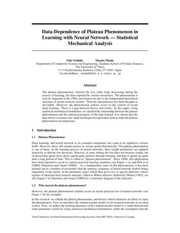
100Training Loss1Training LossTraining 02103Figure 2: Loss curves yielded by student-teacher learning with two-layer perceptron which has 2hidden units, 1 output unit and sigmoid activation, and with (a) IRIS dataset, (b) MNIST dataset, (c)a dataset in R60000 784 drawn from standard normal distribution, as input distribution p(ξ). In everysubfigure, results for 20 trials with random initialization are overlaid. Vanilla SGD (learning rate:(a)(b) 0.005, (c) 0.001) and minibatch size of 1 are used for all three settings.2Formulation2.1Student-Teacher ModelWe consider a two-layer perceptron which has N input units, K hidden units and 1 output unit. WePKdenote the input to the network by ξ RN . Then the output can be written as s i 1 wi g(J i ·ξ) R, where g is an activation function.We consider the situation that the network learns data generated by another network, called “teachernetwork”, which has fixed weights. Specifically, we consider two-layer perceptron that outputsPMt n 1 vn g(B n · ξ) R for input ξ as the teacher network. The generated data (ξ, t) is then fedto the student network stated above and learned by it in the on-line manner (see Figure 3). We assumethat the input ξ is drawn from some distribution p(ξ) every time independently. We adopt vanillastochastic gradient descent (SGD) algorithm for learning. We assume the squared loss functionε 21 (s t)2 , which is most commonly used for regression.2.2Statistical Mechanical FormulationIn order to capture the learning dynamics of nonlinear neural networks described in the previoussubsection macroscopically, we introduce the statistical mechanical formulation in this subsection.Let xi : J i · ξ (1 i K) and yn : B n · ξ (1 n M ). Then (x1 , . . . , xK , y1 , . . . , yM ) N 0, [J 1 , . . . , J K , B 1 , . . . , B M ]T Σ[J 1 , . . . , J K , B 1 , . . . , B M ]holds with N by generalized central limit theorem, provided that the input distribution p(ξ)has zero mean and finite covariance matrix Σ.Next, let us introduce order parameters as following: Qij : J Ti ΣJ j hxi xj i, Rin : J Ti ΣB n hxi yn i, Tnm : B Tn ΣB m hyn ym i and Dij : wi wj , Ein : wi vn , Fnm : vn vm . Then Q R(x1 , . . . , xK , y1 , . . . , yM ) N (0,).RT TThe parameters Qij , Rin , Tnm , Dij , Ein , and Fnm introduced above capture the state of the systemmacroscopically; therefore they are called as “order parameters.” The first three represent the stateof the first layers of the two networks (student and teacher), and the latter three represent theirsecond layers’ state. Q describes the statistics of the student’s first layer and T represents that of theteacher’s first layer. R is related to similarity between the student and teacher’s first layer. D, E, Fis the second layers’ counterpart of Q, R, T . The values of Qij , Rin , Dij , and Ein change duringlearning; their dynamics are what to be determined, from the dynamics of microscopic variables, i.e.connection weights. In contrast, Tnm and Fnm are constant during learning.3
Student mplingξ2Teacher Networkξ1.J1ξ1BMξNε t1(s t)22Figure 3: Overview of student-teacher model formulation.2.2.1Higher-order order parametersThe important difference between our situation and that of Saad and Solla [1995] is the covariancematrix Σ of the input ξ is not necessarily equal to identity. This makes the matter complicated, sincehigher-order terms Σe (e 1, 2, . . .) appear inevitably in the learning dynamics of order parameters.In order to deal with these, here we define some higher-order version of order parameters.(e)(e)(e)(e)Let us define higher-order order parameters Qij , Rin and Tnm for e 0, 1, 2, . . ., as Qij : (e)(e)J Ti Σe J j , Rin : J Ti Σe B n , and Tnm : B Tn Σe B m . Note that they are identical to Qij ,(e)Rin and Tnm in the case of e 1. Also we define higher-order version of xi and yn , namely xi(e)(e)(e)(0)(0)T eT eand yn , as xi : ξ Σ J i , yn : ξ Σ B n . Note that xi xi and yn yn .3Derivation of dynamics of order parametersAt each iteration of on-line learning, weights of the student network J i and wi are updated with KMXXη dεηη wj g(xj ) · wi g 0 (xi )ξ,v n g(yn ) J i [(t s) · wi ]g 0 (xi )ξ N dJ iNNn 1j 1 KMXXη dεηη wi wj g(xj ) ,v n g(yn ) g(xi )(t s) g(xi ) N dwiNNn 1j 1(1)in which we set the learning rate as η/N , so that our macroscopic system is N -independent.(e)(e)Then, the order parameters Qij and Rin (e 0, 1, 2, . . .) are updated with(e) Qij (J i J i )T Σe (J j J j ) J Ti Σe J j J Ti Σe J j J Tj Σe J i J Ti Σe J j"MKXη X(e)(e) Eip g 0 (xi )xj g(yp ) Dip g 0 (xi )xj g(xp )N p 1p 1#MKXX(e)(e)00 Ejp g (xj )xi g(yp ) Djp g (xj )xi g(xp )p 1η2 2 ξ T Σe ξN K,MXp 1"K,KX00Dip Djq g (xi )g (xj )g(xp )g(xq ) p,qEip Ejq g 0 (xi )g 0 (xj )g(yp )g(yq )p,qDip Ejq g 0 (xi )g 0 (xj )g(xp )g(yq ) p,q(e) RinM,MXM,KX#Eip Djq g 0 (xi )g 0 (xj )g(yp )g(xq ) ,p,qTeJ Ti Σe B n J Ti Σe B n (J i J i ) Σ B n "M#KXη X0(e)0(e) Eip g (xi )yn g(yp ) Dip g (xi )yn g(xp ) .N p 1p 1(2)4
Sinceξ T Σe ξ N µe 1where µd : N1 X dλ ,N i 1 iλ1 , . . . , λN : eigenvalues of Σand the right hand sides of the difference equations are O(N 1 ), we can replace these differenceequations with differential ones with N , by taking the expectation over all input vectors ξ:"M(e)KXXdQij(e)(e) ηEip I3 (xi , xj , yp ) Dip I3 (xi , xj , xp )dα̃p 1p 1#MKXX(e)(e) Ejp I3 (xj , xi , yp ) Djp I3 (xj , xi , xp )p 1 η 2 µe 1"K,KXp 1Dip Djq I4 (xi , xj , xp , xq ) p,q K,MXM,MXEip Ejq I4 (xi , xj , yp , yq )(3)p,qDip Ejq I4 (xi , xj , xp , yq ) p,qM,KX#Eip Djq I4 (xi , xj , yp , xq ) ,p,q"M#K(e)XXdRin(e)(e) ηEip I3 (xi , yn , yp ) Dip I3 (xi , yn , xp )dα̃p 1p 1where I3 (z1 , z2 , z3 ) : hg 0 (z1 )z2 g(z3 )i and I4 (z1 , z2 , z3 , z4 ) : hg 0 (z1 )g 0 (z2 )g(z3 )g(z4 )i.(4)In these equations, α̃ : α/N represents time (normalized number of steps), and the brackets h·irepresent the expectation when the input ξ follows the input distribution p(ξ).The differential equations for D and E are obtained in a similar way:"M#KMKXXXXdDij ηEip I2 (xj , yp ) Dip I2 (xj , xp ) Ejp I2 (xi , yp ) Djp I2 (xi , xp ) ,dα̃p 1p 1p 1p 1"M#KXXdEin ηFpn I2 (xi , yp ) Epn I2 (xi , xp )dα̃p 1p 1(5)where I2 (z1 , z2 ) : hg(z1 )g(z2 )i.(6)These differential equations (3) and (5) govern the macroscopic dynamics of learning. In addition,the generalization loss εg , the expectation of loss value ε(ξ) 12 ks tk2 over all input vectors ξ, isrepresented as"M,M#K,KK,MXX11 X2Fpq I2 (yp , yq ) Dpq I2 (xp , xq ) 2Epq I2 (xp , yq ) .εg h ks tk i 22 p,qp,qp,q(7)3.1Expectation termsAbove we have determined the dynamics of order parameters as (3), (5) and (7). However they have(e)expectation terms I2 (z1 , z2 ), I3 (z1 , z2 , z3 ) and I4 (z1 , z2 , z3 , z4 ), where zs are either xi or yn . Bystudying what distribution z follows, we can show that these expectation terms are dependent onlyon 1-st and (e 1)-th order parameters, namely, Q(1) , R(1) , T (1) and Q(e 1) , R(e 1) , T (e 1) ; forexample, (1)(e 1)(1)QiiQijRipZ (e)(e 1) I3 (xi , xj , yp ) dz1 dz2 dz3 g 0 (z1 )z2 g(z3 ) N (z 0, Q(e 1) Rjp )ij(1)Rip5(e 1)Rjp(1)Tpp
holds, where does not influence the value of this expression (see Supplementary Material A.1 formore detailed discussion). Thus, we see the ‘speed’ of e-th order parameters (i.e. (3) and (5)) onlydepends on 1-st and (e 1)-th order parameters, and the generalization error εg (equation (7)) onlydepends on 1-st order parameters. Therefore, with denoting (Q(e) , R(e) , T (e) ) by Ω(e) and (D, E, F )by χ, we can writed (e)Ω f (e) (Ω(1) , Ω(e 1) , χ),dα̃dχ g(Ω(1) , χ),dα̃andεg h(Ω(1) , χ)with appropriate functions f (e) , g and h. Additionally, a polynomial of ΣP (Σ) : dY(Σ λ0i IN ) dXc e Σeλ01 , . . . , λ0dwhereare distinct eigenvalues of Σe 0i 1equals to 0, thus we getΩ(d) d 1Xce Ω(e) .(8)e 0Using this relation, we can reduce Ω(d) to expressions which contain only Ω(0) , . . . , Ω(d 1) , thereforewe can get a closed differential equation system with Ω(0) , . . . , Ω(d 1) and χ.In summary, our macroscopic system is closed with the following order parameters:(0)(1)(d 1)Order variables :Qij , Qij , . . . , Qij,Order constants :(0)(1)(d 1)Tnm, Tnm, . . . , Tnm,(0)(1)(d 1)Rin , Rin , . . . , RinFnm .,Dij , Ein(d: number of distinct eigenvalues of Σ)The order variables are governed by (3) and (5). For the lengthy full expressions of our macroscopicsystem for specific cases, see Supplementary Material A.2.Dependency on input data covariance Σ3.2The differential equation system we derived depends on Σ, through two ways; the coefficient µe 1of O(η 2 )-term, and how (d)-th order parameters are expanded with lower order parameters (as (8)).Specifically, the system only depends on the eigenvalue distribution of Σ.3.3Evaluation of expectation terms for specific activation functionsExpectation terms I2 , I3 and I4 can be analytically determined for some activation functions g,including sigmoid-like g(x) erf(x/ 2) (see Saad and Solla [1995]) and g(x) ReLU(x) (seeYoshida et al. [2017]).4Analysis of numerical solutions of macroscopic differential equationsIn this section, we analyze numerically the order parameter system, derived in the previous section1 .We assume that the second layers’ weights of the student and the teacher, namely wi and vn , are fixedto 1 (i.e. we consider the learning of soft-committee machine), and that K and M are equal to 2, forsimplicity. Here we think of sigmoid-like activation g(x) erf(x/ 2).4.1Consistency between macroscopic system and microscopic systemFirst of all, we confirmed the consistency between the macroscopic system we derived and the originalmicroscopic system. That is, we computed the dynamics of the generalization loss εg in two ways:(i) by updating weights of the network with SGD (1) iteratively, and (ii) by solving numerically thedifferential equations (5) which govern the order parameters, and we confirmed that they accord witheach other very well (Figure 4). Note that we set the initial values of order parameters in (ii) as valuescorresponding to initial weights used in (i). For dependence of the learning trajectory on the initialcondition, see Supplementary Material A.3.1We executed all computations on a standard PC.6
Generalization loss g100(a)Microscopic (N 100)10010110110210210310310 4 0(b)10 4 malized Steps /NFigure 4: Example dynamics of generalization error εg computed with (a) microscopic and (b)macroscopic system. Network size: N -2-1. Learning rate: η 0.1. Eigenvalues of Σ: λ1 0.4 withmultiplicity 0.5N , λ2 1.2 with multiplicity 0.3N , and λ3 1.6 with multiplicity 0.2N . Blacklines: dynamics of εg . Blue lines: Q11 , Q12 , Q22 . Green lines: R11 , R12 , R21 , R22 .4.2Case of scalar input covariance Σ σINAs the simplest case, here we consider the case that the convariance matrix Σ is proportional tounit matrix. In this case, Σ has only one eigenvalue λ µ1 of multiplicity N , then our orderparameter system contains only parameters whose order is 0 (e 0). For various values of µ1 , wesolved numerically the differential equations of order parameters (5) and plotted the time evolutionof generalization loss εg (Figure 5(a)). From these plots, we quantified the lengths and heights ofthe plateaus as following: we regarded the system is plateauing if the decreasing speed of log-loss issmaller than half of its terminal converging speed, and we defined the height of the plateau as themedian of loss values during plateauing. Quantified lengths and heights are plotted in Figure 5(b)(c).It indicates that the plateau length and height heavily depend on µ1 , the input scale. Specifically, asµ1 decreases, the plateau rapidly becomes longer and lower. Though smaller input data lead to longerplateaus, it also becomes lower and then inconspicuous. This tendency is consistent with Figure2(a)(b), since IRIS dataset has large µ1 ( 15.9) and MNIST has small µ1 ( 0.112). Consideringthis, the claim that the plateau phenomenon does not occur in learning of MNIST is controversy; thissuggests the possibility that we are observing quite long and low plateaus.Note that Figure 5(b) shows that the speed of growing of plateau length is larger than O(1/µ1 ). Thisis contrast to the case of linear networks which have no activation; in that case, as µ1 decreases thespeed of learning gets exactly 1/µ1 -times larger. In other words, this phenomenon is peculiar tononlinear networks.(b)(a)(c)Figure 5: (a) Dynamics of generalization error εg when input variance Σ has only one eigenvalueλ µ1 of multiplicity N . Plots with various values of µ1 are shown. (b) Plateau length and (b)plateau height, quantified from (a).7
4.3Case of different input covariance Σ with fixed µ1In the previous subsection we inspected the dependence of the learning dynamics on the first momentµ1 of the eigenvalues of the covariance matrix Σ. In this subsection, we explored the dependence ofthe dynamics on the higher moments of eigenvalues, under fixed first moment µ1 .In this subsection, we consider the case in which the input covariance matrix Σ has two distinctnonzero eigenvalues, λ1 µ1 λ/2 and λ2 µ1 λ/2, of the same multiplicity N/2 (Figure6). With changing the control parameter λ, we can get eigenvalue distributions with various valuesof second moment µ2 hλ2i i.Δλμ1 Δλ2μ1 Δλ2λFigure 6: Eigenvalue distribution with fixed µ1 parameterized by λ, which yields various µ2 .Figure 7(a) shows learning curves with various µ2 while fixing µ1 to 1. From these curves, wequantified the lengths and heights of the plateaus, and plotted them in Figure 7(b)(c). These indicatethat the length of the plateau shortens as µ2 becomes large. That is, the more the distribution ofnonzero eigenvalues gets broaden, the more the plateau gets alleviated.(b)(a)(c)Figure 7: (a) Dynamics of generalization error εg when input variance Σ has two eigenvaluesλ1,2 µ1 λ/2 of multiplicity N/2. Plots with various values of µ2 are shown. (b) Plateau lengthand (c) plateau height, quantified from (a).5ConclusionUnder the statistical mechanical formulation of learning in the two-layered perceptron, we showedthat macroscopic equations can be derived even when the statistical properties of the input aregeneralized. We showed that the dynamics of learning depends only on the eigenvalue distributionof the covariance matrix of the input data. By numerically analyzing the macroscopic system, it isshown that the statistics of input data dramatically affect the plateau phenomenon.Through this work, we explored the gap between theory and reality; though the plateau phenomenonis theoretically predicted to occur by the general symmetrical structure of neural networks, it isseldom observed in practice. However, more extensive researches are needed to fully understand thetheory underlying the plateau phenomenon in practical cases.8
AcknowledgementThis work was supported by JSPS KAKENHI Grant-in-Aid for Scientific Research(A) (No.18H04106).ReferencesFlorent Cousseau, Tomoko Ozeki, and Shun-ichi Amari. Dynamics of learning in multilayer perceptrons near singularities. IEEE Transactions on Neural Networks, 19(8):1313–1328, 2008.Kenji Fukumizu and Shun-ichi Amari. Local minima and plateaus in hierarchical structures ofmultilayer perceptrons. Neural Networks, 13(3):317–327, 2000.Sebastian Goldt, Madhu S Advani, Andrew M Saxe, Florent Krzakala, and Lenka Zdeborová.Dynamics of stochastic gradient descent for two-layer neural networks in the teacher-student setup.arXiv preprint arXiv:1906.08632, 2019.Weili Guo, Yuan Yang, Yingjiang Zhou, Yushun Tan, Haikun Wei, Aiguo Song, and Guochen Pang.Influence area of overlap singularity in multilayer perceptrons. IEEE Access, 6:60214–60223,2018.Kazuyuki Hara, Daisuke Saitoh, and Hayaru Shouno. Analysis of dropout learning regarded asensemble learning. In International Conference on Artificial Neural Networks, pages 72–79.Springer, 2016.John Milnor. On the concept of attractor. In The Theory of Chaotic Attractors, pages 243–264.Springer, 1985.A Emin Orhan and Xaq Pitkow.arXiv:1701.09175, 2017.Skip connections eliminate singularities.arXiv preprintHyeyoung Park, Shun-ichi Amari, and Kenji Fukumizu. Adaptive natural gradient learning algorithmsfor various stochastic models. Neural Networks, 13(7):755–764, 2000.Peter Riegler and Michael Biehl. On-line backpropagation in two-layered neural networks. Journalof Physics A: Mathematical and General, 28(20):L507, 1995.David Saad and Sara A Solla. On-line learning in soft committee machines. Physical Review E, 52(4):4225, 1995.Michiel Straat and Michael Biehl. On-line learning dynamics of relu neural networks using statisticalphysics techniques. arXiv preprint arXiv:1903.07378, 2019.Michiel Straat, Fthi Abadi, Christina Göpfert, Barbara Hammer, and Michael Biehl. Statisticalmechanics of on-line learning under concept drift. Entropy, 20(10):775, 2018.Shiro Takagi, Yuki Yoshida, and Masato Okada. Impact of layer normalization on single-layerperceptron—statistical mechanical analysis. Journal of the Physical Society of Japan, 88(7):074003, 2019.Haikun Wei, Jun Zhang, Florent Cousseau, Tomoko Ozeki, and Shun-ichi Amari. Dynamics oflearning near singularities in layered networks. Neural computation, 20(3):813–843, 2008.Yuki Yoshida, Ryo Karakida, Masato Okada, and Shun-ichi Amari. Statistical mechanical analysisof online learning with weight normalization in single layer perceptron. Journal of the PhysicalSociety of Japan, 86(4):044002, 2017.Yuki Yoshida, Ryo Karakida, Masato Okada, and Shun-ichi Amari. Statistical mechanical analysisof learning dynamics of two-layer perceptron with multiple output units. Journal of Physics A:Mathematical and Theoretical, 2019.9
The statistical property of data just can affect the learning dynamics dramatically; for example, see Figure 2 for learning curves with using different datasets and same network architecture. We focus on what kind of statistical property of the data brings plateau phenomenon. 0 250 500 750 1000 Epoch 0.00 0.25 0.50 0.75 1.00 1.25 1.50 Training .