Transcription
Rainfall Modeling and Simulation1IntroductionThe payout and price of a rainfall-based index insurance contract are both functions of rainfall, which isa random process. In order to design and price these contracts, therefore, the buyers and the sellers ofthe contracts must both have a satisfactory understanding of the rainfall process, and must be able tocommunicate their beliefs to each other in order to negotiate the design and price of the contract. Ratherthan base a contract design on the empirical (historical) distributions of various rainfall statistics, such asthe 10th percentile of seasonal rainfall, or the length of the longest dry spell in the season, which can besensitive to individual, unusual historical events and further limited by sparse or missing data, the designersof insurance contracts can use statistical models trained on historical data to more accurately estimatethe distributions of various rainfall-based statistics. A statistical model for rainfall has at least two usefulproperties: (1) it can describe the relationship between rainfall at a given location and other weather-relatedvariables, such as large-scale climate variables and rainfall observed at other nearby locations, in order toreduce the unexplained variation in rainfall amounts, and (2) it provides a principled way to quantify theuncertainty that accompanies rainfall processes, which is crucial to the efficient design of insurance contracts.This document will review and discuss different statistical models used for rainfall, and different strategiesfor evaluating these models and simulating rainfall from them. We pay particular attention to the way inwhich low-rainfall events are modeled, because the main purpose of these contracts is to allow farmers tohedge their risk of poor yields due to drought. Many of the models we discuss, though, could also be used toinvestigate properties of floods, or be used to simulate rainfall time series as inputs to crop growth models.We believe that there is currently a gap in the knowledge between how rainfall simulators generally work,and how they work specifically in the context of index insurance. We recommend that further research befocused on filling in this knowledge gap, and we provide some guidelines in Section 3 for how this can bedone.2Rainfall ModelsWe will review four basic types of rainfall models that have been the focus of most of the recent researchon rainfall modeling: (1) Generalized linear models (GLMs), (2) Hidden Markov models (HMMs), (3)Nonparametric models, and (4) “Mechanistic” models. The first three types are reviewed in Wilks andWilby (1999), and the first and fourth types are reviewed in Chandler, et al. (2007).2.1GLMsCoe and Stern (1982) and Stern and Coe (1984) first introduced the use of GLMs to model a daily timeseries of rainfall measurements at a single site. These types of models are the simplest example of stochasticweather models, and were the first to be widely used. GLMs are parametric models that have the structureto condition the outcome variable, daily rainfall, on observed covariates, such as sine and cosine functionsof time, to account for seasonality, climatological variables such as sea surface temperature, and regionalforecasts. Multiple sites can be modeled this way using multivariate time series methods, where correlationsacross space are modeled, and rainfall outcomes at locations that were not observed can be imputed. Themarginal distribution of daily rainfall data has a point mass at zero (dry days), so it is common for thesemodels to be comprised of two parts: (1) a model for dependent binary data - such as a two-state Markovchain model - to model the occurrence of rainfall on a given day, conditional on previous rainfall occurence,1
and (2) a right-skewed distribution, such as the exponential, gamma, or mixed exponential distribution, tomodel the intensity of rainfall on wet days. Sine and cosine functions of different periods can be includedor excluded according to formal tests such as likelihood ratio tests; the most obvious source of seasonalityis the yearly rotation of the earth, although lower and higher-frequency sources of seasonality drive rainfallprocesses as well, such as ENSO state, which occurs at a period of 3-7 years, and various local atmosphericconditions, which can occur on periods of one month or shorter. One of the strengths of GLMs is thatthey can account for climate change over a long time scale through their incorporation of covariate effects.Most GLMs are fit using maximum-likelihood methods (McCullagh and Nelder, 1989), although Bayesianmethods can also be used.2.2HMMsThe second type of model is an HMM, which is also fit to discrete data in time and space, but differsfrom a GLM in that it models autocorrelation and spatial correlation through some number, K, of discrete,unobserved hidden states, which correspond to different “weather states” that result in different patterns ofrainfall. In an HMM, the hidden states change through time according to a first-order Markov chain, and theoutcomes are modeled as independent draws from distributions conditional on their corresponding hiddenstates. Basic HMMs, which are stationary in time, have been extended to model non-stationary processes byincorporating time-varying covariates (i.e. sine and cosine functions of time, seasonal forecasts, etc.); thesemodels are called non-homogeneous HMMs, or NHMMs. The first NHMMs for rainfall data, introducedby Hughes and Guttorp (1994a,b) and extended in Hughes et al. (1999), allowed for seasonality in therainfall occurrence process, whereas more recent work (Bellone et al., 2000, Robertson et al., 2004, 2006) hasallowed for seasonality in the rainfall amounts process (i.e. the conditional distributions) as well. NHMMscan be fit using the EM algorithm or Bayesian methods; in either case, they are fit given a pre-determinedvalue of K, the number of hidden states. The choice of K can be guided in part by (1) out-of-samplepredictive error measured via cross-validation, and (2) scientific grounds in which the hidden states havespecific interpretations in the context of the application. The autocorrelation structure of HMMs can bemade richer by allowing higher-order dependence in the hidden state sequence, or by relaxing the conditionalindependence of observations. The strength of NHMMs for rainfall data lies in their ability to reflect realscientific phenomena, like regional atmospheric conditions, with the hidden states.2.3Nonparametric ModelsNonparametric models for rainfall represent an interesting alternative to GLMs and HMMs, because theirlack of dependence on parametric distributions to describe the data gives them flexibility to model certainfeatures of the rainfall process better than other models. The key feature of most nonparametric modelsis a resampling algorithm, in which daily time series of rainfall are simulated by resampling the observeddata in a way that accounts for the autocorrelation of observed rainfall as well as the relationships betweenrainfall and other weather variables. Such models have been developed and fit by Young (1994), Lall et al.(1996), Rajagopalan & Lall (1999), and Moron et al. (2008). Nonparametric models generally can moreflexibly describe nonlinear relationships between variables, but are sometimes limited in that they can onlyreproduce values that have already been observed, which limit their ability to incorporate the effects oflong-term climate changes into the rainfall process.2.4Mechanistic ModelsThe fourth type of model in current use is one that models the physical process of rainfall using radar datacollected at a high resolution in time and space. These models describe a process by which ’rain events’occur randomly, and spawn smaller ’storms’ at random times and locations within their interiors (which are2
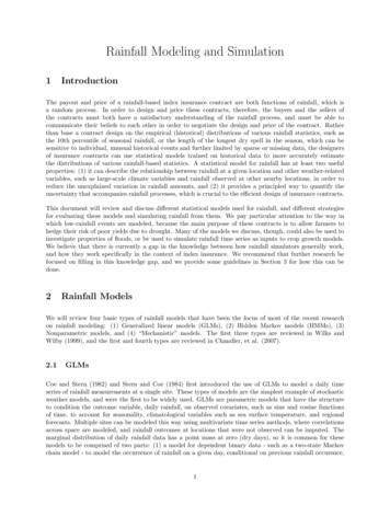
typically regions of over 1000 km2 ), which in turn are comprised of ’rain cells’ which also arise at randomtimes and locations within the storm. The entire rain event moves across space at a random velocity. Theresolution of data to which these models are fit is typically high with respect to both space (2 km2 regions)and time (5 minute intervals) (Chandler, et al., 2007). These models are stationary in time, and are usuallyfit with the goal of describing floods in catchment areas. Two drawbacks of these models with respect toindex insurance applications are that (1) they are not well-suited to incorporating covariates that couldexplain variation in rainfall over long time periods, and (2) they require high-resolution radar data to be fit,and this data is unavailable for most developing countries in which index insurance is being used. For thesereasons, we don’t focus on mechanistic models in this report.3Rainfall SimulationNo matter what type of model is fit, a common goal is to simulate rainfall from the fitted model. Suchsimulations should be produced by incorporating two sources of variation: (1) variation built into the model,and (2) variation associated with the uncertainty with which the parameters of the model are estimatedduring the training phase of the data analysis. This second source of variation is often overlooked. (Athird source of variation could be considered: the choice of the model itself - but we don’t discuss this issuehere). Although Bayesian methods are not widely used in rainfall modeling thus far, they offer a natural andconvenient way to simulate rainfall while incorporating both of the above sources or variability by samplingfrom the posterior predictive distribution of the outcome variable (Gelman, et al. 2004).A crucial fact about index insurance design is that the payout and price are complicated, but deterministic,functions of rainfall. The payout, for example, is a random variable which is realized once per year, and itsdistribution depends entirely on the parameters of the rainfall model (and the parameters of the contract,which we treat as fixed, for now). The goodness-of-fit of rainfall models is usually checked with respectto monthly means and variances, and the lengths of runs of wet and dry spells. Mavromatis and Hansen(2001) compare a group of stochastic weather generators, paying special attention to their goodness-of-fitwith respect to the interannual variability of rainfall, which is known to be somewhat difficult to capturewith statistical models. In this section we will outline steps needed to be taken in order to evaluate thegoodness-of-fit of rainfall models with respect to the particular characteristics of rainfall that influence thepayout of an index insurance contract illustrated in Osgood, et al. (2007).Consider an index insurance contract for a single site with the following design: Dekadal sums of rainfallare calculated, and then, based on a sowing condition that stipulates that the growing season starts in thefirst dekad to receive more than s mm of rainfall, 3 contract phases are determined, each of which lasts2-4 dekads and corresponds to a different part of the growth of the specific crop for which the contract isdesigned. In each phase, the payout function is a piecewise linear function of the sum of rainfall during thephase, such as the one illustrated in Figure 1(a). Given the parameters of the contract (sowing condition,phase definitions, and the parameters of the piecewise linear phase payout functions), the payout for a givenyear is a random variable that we observe: the sum of the payouts from each phase. If we have N yearsof data, then we observe N realizations of payouts, where N is typically between 5 and 50 for sites thatimplement index insurance. Considering that efficient insurance designs only pay out approximately 10-20%of the time, then even for a relatively long time series, such as a 50-year series, we may only observe 5 to10 non-zero payouts: many too few observations to estimate the mean or 99th percentile of a distribution,which are critical factors in the price of insurance (Osgood, et al., 2007).To estimate the distribution of payouts more accurately we fit a model to daily data and simulate thousandsof years of data. Before we check these simulated payouts against the observed payouts, we recommendperforming a series of intermediate goodness-of-fit model checks of statistics that are components of theinsurance payout. These statistics to check include:1. Dekadal sums. Check that the model produces dekadal sums with approximately the same distribution3
(a) Payout Function(b) Payout (200) 0.5%DensityPayout150100P(0) 95%P(shaded area) 4.5%Exit 5050Trigger 120001002003004005000Phase Sum (mm)50100150200PayoutFigure 1: The payout function and distribution for a hypothesized distribution of rainfall by phase. (a) Theleft plot shows a (normal) distribution of rainfall, with the payout plotted on the y-axis as a function of therainfall, plotted on the x-axis. The shaded area is the proportion of years in which there is a payout for thisphase, and the darkly shaded area is the proportion of years in which there is a maximum payout for thisphase. (b) In the right plot, the hypothetical distribution of the payout is depicted. There is a point mass atzero and at the maximum payout (200). The interior of the distribution is a truncated normal distribution.of the observed dekadal sums, for each dekad of the year.2. The onset of the growing season. Check that the model-based estimates of the start of the growingseason are in line with the observed sowing dekads.3. Phase sums. The phase sum is the sum of 2-4 dekads of rainfall. Dekadal sums may be correlatedwithin the growing season, so even a good model for dekadal sums may be bad for phase sums if itignores correlations between dekads.4. The lower tail of phase sums. Most contracts are designed to pay out in approximately 10-20% ofyears. In other words, the triggers for each phase of most contracts are set to low quantiles of thephase sum distributions. We must pay special attention to the fit of models with respect to these lowquantiles of the phase sum distributions to ensure that the payout distributions are well-estimated.Using Bayesian methods, the formal name for an analysis of these kinds is a posterior predictive check(Gelman, et al. 1996). Note that one must check the goodness-of-fit of not only statistics that are explicitlymodeled, but also of those that aren’t. Generally speaking, if the residuals from a rainfall model are spatiallyclustered, or are related to other observable weather variables, then a buyer or seller of a rainfall contractbased on such a model could factor in these additional variables and “game the system” to his advantage.In conclusion, we stress that developing a model for rainfall from which we can make accurate inferences aboutlow-rainfall events, for the purpose of designing and pricing an index insurance contract, is a challengingprocess that has received much attention already, and deserves still more.4ReferencesBellone, E., Hughes, J.P., and Guttorp,P. A Hidden Markov Model for Downscaling Synoptic AtmosphericPatterns to Precipitation Amounts (2000). Climate Research, 15:1-12.4
Chandler, R.E., Isham, V., Bellone, E., Yang, C., and Northrop, P. (2007) Space-time modelling of rainfallfor continuous simulation, in Statistical Methods for Spatio-Temporal Systems, ed. Finenstadt, B., Held, L.,and Isham, V. Chapman & Hall, London.Coe, R. and Stern, R.D. (1982). Fitting models to daily rainfall. J. Appl. Meteorol., 21:1024-1031.Gelman, A., Meng, X-L., Stern, H.S. (1996). Posterior predictive assessment of model fitness via realizeddiscrepancies (with discussion). Statistica Sinica, 6:733-807.Gelman, A., Carlin, J.B., Stern, H.S., and Rubin, D.B. (2004). Bayesian Data Analysis. Chapman & Hall,London.Hughes, J.P. and Guttorp, P. (1994a). Incorporating spatial dependence and atmospheric data in a modelof precipitation. J. Apppl. Meteorol., 33:1503-1515.Hughes, J.P. and Guttorp, P. (1994b). A class of stochastic models for relating synoptic atmospheric patternsto regional hydrologic phenomena. Water Resources Research, 30: 1535:1546.Hughes, J.P., Guttorp, P. and Charles, S.P. (1999). A non-homogeneous hidden Markov model for precipitation occurrence. J. Royal Stat. Soc.: Series C, 48:15-30.Lall, U., Rajagopalan, B., and Tarboton, D.G. (1996) A nonparametric wet/dry spell model for resamplingdaily precipitation. Water Resources Research, 32:2803-2823.Lall, U., and Sharma, A. (1996). A nearest-neighbor bootstrap for resampling hydrological time series.Water Resources Research, 32:679-693.Mavromatis, T., and Hansen, J.W. (2001). Interannual variability characteristics and simulated crop response of four stochastic weather generators, Agricultural and Forest Methodology, 109: 283-296.McCullagh, P. and Nelder, J. (1989). Generalized Linear Models (second edition). Chapman & Hall, London.Moron, V., Robertson, A.W., Ward, M.N., and Ndiaye, O. (2008). Weather types and rainfall over Senegal.Part II: Downscaling of GCM simulations. Journal of Climate, 21:288-307.Osgood, D.E., McLaurin, M., Carriquiry, M., Mishra, A., Fiondella, F., Hansen, J., Peterson, N., and Ward,N. (2007). Designing Weather Insurance Contracts for Farmers in Malawi, Tanzania, and Kenya, FinalReport to the Commodity Risk Management Group, ARD, World Bank. International Research Institutefor Climate and Society (IRI), Columbia University, New York, USA.Robertson, A.W., Kirshner, S. and Smyth, P. (2004). Downscaling of daily rainfall occurrence over NortheastBrazil using a Hidden Markov Model. J. Climate, 17:4407-4424.Robertson, A.W., Kirshner, S., Smyth, P., Charles, S.P., and Bates, B.C. (2006). Subseasonal-to-interdecadalvariability of the Australian monsoon over North Queensland. Q. J. R. Meteorol. Soc., 132:519-542.Stern, R.D. and Coe, R. (1984). A model fitting analysis of rainfall data (with discussion). J. Roy. Stat.Soc.: Series A, 147:1-34.Wilks, D.S. and Wilby, R.L. (1999). The weather generation game: a review of stochastic weather models.Progress in Physical Geography, 23, 3:329-357.Young, K.C. (1994). A multivariate chain model for simulating climatic parameters from daily data. Journalof Applied Meteorology, 33:661-671.5
long-term climate changes into the rainfall process. 2.4 Mechanistic Models The fourth type of model in current use is one that models the physical process of rainfall using radar data collected at a high resolution in time and space. These models describe a process by which 'rain events'