Transcription
JOURNAL OF GEOPHYSICAL RESEARCH, VOL. 110, D21104, doi:10.1029/2005JD005763, 2005Diurnal cycle of tropical precipitationin Tropical Rainfall Measuring Mission (TRMM)satellite and ocean buoy rain gauge dataKenneth P. Bowman, J. Craig Collier, Gerald R. North, Qiaoyan Wu, and Eunho Ha1Department of Atmospheric Sciences, Texas A&M University, College Station, Texas, USAJames Hardin2College of Science, Texas A&M University, College Station, Texas, USAReceived 7 January 2005; revised 29 June 2005; accepted 1 August 2005; published 4 November 2005.[1] The climatological diurnal cycle of precipitation in the tropics is analyzed using datafrom rain gauges on ocean buoys and satellite measurements by the Tropical RainfallMeasuring Mission (TRMM) satellite. The ocean buoy data are from the NOAA/PacificMarine Environmental Laboratory Tropical Atmosphere-Ocean/Triangle Trans-Oceanbuoy Network in the tropical Pacific Ocean. TRMM data are from the precipitation radar(PR) and the TRMM microwave imager (TMI). Climatological hourly mean precipitationrates are analyzed in terms of the diurnal and semidiurnal harmonics. Both data setsconfirm an early morning peak in precipitation over ocean regions. The amplitude of thediurnal harmonic over the oceans is typically less than 25% of the mean precipitation rate.Over tropical land masses the rainfall peaks in the afternoon and evening hours. Therelative amplitude of the diurnal harmonic over land is larger than over the ocean, oftenexceeding 50% of the mean rain rate. Previously noted differences between the TMI andPR rainfall retrievals persist in the diurnal cycle. On average the TMI measures morerainfall than the PR and has a larger diurnal variation. Phase differences between the twoinstruments do not show a consistent bias.Citation: Bowman, K. P., J. C. Collier, G. R. North, Q. Wu, E. Ha, and J. Hardin (2005), Diurnal cycle of tropical precipitation inTropical Rainfall Measuring Mission (TRMM) satellite and ocean buoy rain gauge data, J. Geophys. Res., 110, D21104,doi:10.1029/2005JD005763.1. Introduction[2] Simulation of clouds and precipitation has proven tobe one of the most difficult problems in modeling theEarth’s climate system. Dynamics, thermodynamics, andradiation all play important roles in cloud and precipitationsystems. Such systems are highly nonlinear and span a hugerange of scales from the synoptic to the microphysical.Incomplete understanding of the processes that controlclouds and precipitation, and of the climate feedbacksinvolving clouds, is one of the largest sources of uncertaintyin predictions of possible future anthropogenic climatechange.[3] The Earth’s weather and climate vary both regularlyand irregularly. Regular variations are due, for example, toperiodic external forcing by the annual and diurnal cycles ofsolar radiation. The characteristics of the forcing at diurnaland annual frequencies in terms of top-of-the-atmosphere1Permanently at Department of Information and Statistics, YonseiUniversity, Wonju, Korea.2Now at Department of Epidemiology and Biostatistics, University ofSouth Carolina, Columbia, South Carolina, USA.Copyright 2005 by the American Geophysical Union.0148-0227/05/2005JD005763 09.00insolation are well known, so simulations of the climate atthose frequencies provide a valuable means of testing ourunderstanding of the response of the climate to directforcing. In addition, the periodic forcing by solar radiationis known to produce different diurnal responses over thecontinents and oceans. The two environments thus provide,in effect, two different planets that can be used to validatemodels.[4] Evaluation of model simulations of the annual anddiurnal cycles requires observational data for comparison.Here we use remotely sensed data from the TropicalRainfall Measuring Mission (TRMM) satellite and in situdata from rain gauges on the National Oceanic andAtmospheric Administration/Pacific Marine EnvironmentLaboratory (NOAA/PMEL) Tropical Atmosphere Ocean/Triangle Trans-Ocean buoy Network (TAO/TRITON) buoyarray in the tropical Pacific Ocean to develop statisticalestimates of the diurnal cycle in tropical precipitation. Thebuoy data have the important characteristic that they arenot influenced by the local thermodynamic or orographiceffects to which rain gauges located on islands are subjected [Reed, 1980].[5] There is an extensive history of observational andmodel studies of the diurnal cycle of precipitation. Convective precipitation over land during the warm season tends toD211041 of 14
D21104BOWMAN ET AL.: DIURNAL CYCLE OF TROPICAL PRECIPITATIONpeak in the late afternoon to early evening hours and isthought to be a direct response to daytime heating of thesurface and the planetary boundary layer: Heating of thelower atmosphere produces available potential energy thatcan be released by convective overturning. Wallace [1975]reviewed some earlier studies of the diurnal cycle andanalyzed the diurnal cycle of precipitation and thunderstorm activity over the United States using rain gauge data.He concluded that daytime surface heating provides thelarge-scale thermodynamic control of convection and precipitation but that dynamical effects in some regions cansubstantially change the phase of convection from lateafternoon to midnight or even early morning hours.Wallace [1975] was apparently thinking of large-scaleboundary layer processes as the predominant dynamicalinfluence, but the growth and propagation of mesoscalesystems initially triggered by diurnal heating also affectthe timing of the peak precipitation [Carbone et al., 2002;Rickenbach, 2004; Nesbitt and Zipser, 2003].[6] The diurnal cycle of precipitation is typically differentover the oceans than over land. At most oceanic locationsthe maximum precipitation tends to occur in the earlymorning hours (typically between 0300 and 0600 LT).Kraus [1963] analyzed midlatitude weather ship data andfound more frequent precipitation at night. He argued thatthis counterintuitive diurnal cycle is due to the stabilizingeffects of solar heating of cloud tops during the day or,equivalently, the destabilizing effects of nighttime radiativecooling at cloud tops. Gray and Jacobson [1977] studiedprecipitation in the tropics, primarily using rain gauge datafrom a small set of islands, and found an early morningmaximum in deep convection and precipitation. Theyargued that the early morning maximum was the result ofheating differences between organized cloud systems andsurrounding clear regions. They also noted that while largerislands have an early morning precipitation maximum, theyalso have an even larger afternoon maximum, which theyattributed to daytime heating of the land surface.[7] Randall et al. [1991] used a global climate model(GCM) to simulate the diurnal cycle of precipitation. Theyfound that a diurnal cycle exists over the oceans even on anall-water planet. From controlled experiments with theGCM they concluded that stabilization of the atmospherethrough absorption of solar radiation by clouds is thedominant process responsible for the diurnal cycle, assuggested by Kraus [1963]. They also found that a radiatively forced diurnal cycle exists in a one-dimensionalcolumn model even when there is no diurnal forcing ofthe large-scale vertical motion field, which argues againstthe hypothesis of Gray and Jacobson [1977].[8] The Global Atmospheric Research Program (GARP)Atlantic Tropical Experiment (GATE) in 1974 provided oneof the first extensive data sets of tropical oceanic precipitation not based on island rain gauge data. A number ofstudies examined the diurnal cycle in the GATE data andfound an afternoon maximum in precipitation, which contradicted studies at other locations [Gray and Jacobson,1977; McGarry and Reed, 1978; Albright et al., 1981]. Theprecipitation during GATE phase III was dominated by asmall number of squall lines propagating through theobserving area. Because the GATE observing period wasrelatively short, it is difficult to say whether the diurnalD21104phase of the squall lines was influenced by the small samplesize. It is interesting to note that an afternoon peak wasfound during phases I and III but a morning peak occurredduring phase II. A later study by Reed and Jaffe [1981],using Meteosat IR imagery, found that an afternoon peak incold clouds also occurred over the GATE area in 1978, so itis possible that the eastern tropical Atlantic is affected bythe proximity to the African coast. That is, squall lines weretriggered by the coastal sea breeze circulation or deepconvection over West Africa.[9] Over the years a number of authors have used tropicalcold cloud occurrence from IR satellite data or precipitationamounts inferred from the IR data to study the diurnal cycle[Reed and Jaffe, 1981; Albright et al., 1985; Hendon andWoodberry, 1993; Janowiak et al., 1994; Yang and Slingo,2001]. The advantages of geostationary IR data are highhorizontal and temporal resolutions; the principal disadvantages are the indirect relationship of the measurement toprecipitation rates and the lack of a signal in areas that havelittle deep convection. Albright et al. [1985] found that inJanuary and February of 1979 in the tropical Pacific, mostlocations had an early morning peak in convective cloudiness. The exception was the South Pacific ConvergenceZone (SPCZ), which also exhibited an afternoon peak.Hendon and Woodberry [1993] generally found an afternoon or early evening peak in deep convective activity overthe continents and a morning peak over the oceans, including the SPCZ. Janowiak et al. [1994] found similar results.Yang and Slingo [2001] compared the observed diurnalcycle with simulations by the UK Met Office Unified Modeland noted a number of problems with simulating the phaseof the diurnal cycle.[10] Several authors have used data from passive microwave satellite instruments such as the Special SensorMicrowave/Imager (SSM/I) to study the diurnal cycle overthe tropical oceans. Microwave emission is more directlyrelated to precipitation rate than is cloud top temperature[Wilheit et al., 1977]. Because the SSM/I instruments haveflown on Sun-synchronous satellites, it is not possible toestimate the diurnal cycle reliably from a single satellite.Chang et al. [1995] used SSM/I data from multiple satelliteswith different equator crossing times to estimate the diurnalcycle of oceanic precipitation. They found an early morningpeak in precipitation at most locations, although the uncertainty in their estimates was large. The TRMM satellite is ina non-Sun-synchronous orbit. During its precession periodit samples rainfall at different times throughout the diurnalcycle. Nesbitt and Zipser [2003] identified individual stormsand mesoscale systems in the TRMM data and analyzedrain rate versus time of day, stratified by the type ofprecipitation feature. Over tropical land they found anafternoon peak, while ocean locations showed an earlymorning peak and a weaker diurnal cycle. They also foundthat the early morning peak is due to increased numbers ofprecipitating features rather than increased rain intensity.Collier and Bowman [2004] compared the diurnal cycleinferred from 4 years of TRMM data with simulations bythe National Center for Atmospheric Research (NCAR)Community Climate Model version 3. They noted a numberof problems with the model’s simulation of the diurnalcycle, including both amplitude and phase errors. Dai andTrenberth [2004] analyzed the diurnal cycle in the NCAR2 of 14
D21104BOWMAN ET AL.: DIURNAL CYCLE OF TROPICAL PRECIPITATIONCommunity Climate System Model and compared precipitation frequencies with surface observations [Dai, 2001].They also found significant differences between observations and simulations.[11] Serra and McPhaden [2004] examined the diurnalcycle of various precipitation parameters using the TAO/TRITON ocean buoy rain gauge data. They found an earlymorning maximum in precipitation amount, intensity, andfrequency. In this study, we use the buoy data, along withmore than 6 years of TRMM rainfall data, to study thediurnal cycle in rainfall rates. The goals of this research areto establish confidence limits on the amplitude and phase ofthe diurnal cycle for both buoy and satellite data, tocompare the diurnal cycles observed by the two systems,and to analyze differences between the diurnal cycle measured by the two primary TRMM precipitation instruments,the precipitation radar (PR) and the TRMM microwaveimager (TMI).2. Data2.1. TRMM Data2.1.1. Satellite and Instruments[12] The TRMM satellite is a joint U.S.-Japan missionthat was launched in November 1997. Designed to observeprecipitation in the tropics, it operates in a low-inclination(35 ), low-altitude orbit. During the first 3 or more years ofoperation, TRMM flew at an altitude of 350 km. InAugust 2001 the orbit was boosted to 400 km to reducedrag, and thus fuel use, and to increase the lifetime ofthe mission. TRMM has significantly outlasted its nominal3-year design lifetime. Details of the TRMM mission andinstruments are given by Simpson et al. [1988] andKummerow et al. [1998, 2000].[13] The TRMM satellite measures precipitation withboth the precipitation radar and the TRMM microwaveimager. The PR and the launch vehicle were provided byJapan. The other instruments and the spacecraft wereprovided by the United States. The PR is a phased-arrayradar operating at 13.8 GHz ( 2.1 cm wavelength). Theobserving footprint is 4 4 km at nadir, and the verticalresolution is 250 m. The radar scans perpendicular to thesatellite motion with a swath width of 220 km. Because ofthe comparatively narrow swath the mean sampling intervalfor PR measurements at the equator is roughly 2 to 3 days.[14] The TMI is a multichannel, dual-polarization, passive microwave radiometer based on the SSM/I instrumentsused on the operational Defense Meteorological SatelliteProgram polar orbiters. The TMI uses an offset antenna toscan the Earth’s surface in a conical pattern across thesatellite’s flight track. This scanning pattern is designed tomaintain a constant viewing angle at the Earth’s surface.This design eliminates variations in emitted radiation due toviewing angle dependence of the surface microwave emissivity. The size of the instrument’s field of view depends onthe frequency, ranging from 63 37 km at 10.65 GHz to7 5 km at 85.5 GHz. The TMI swath width is 780 km,which means that the mean sampling interval at the equatoris about 1 day. Precipitation retrieval algorithms over theocean rely primarily on emission of microwave radiationfrom hydrometeors observed against the relatively coldbackground provided by the low-emissivity ocean surface.D21104Because of variations in the surface emissivity, rainfallretrievals over land are based on the ice scattering signalsin the high-frequency (85 GHz) channel, while the oceanretrieval algorithm uses the ice scattering information in the85 GHz channels to select rain profiles [Kummerow et al.,2001]. As a result, the retrieval algorithms over land andocean are substantially different, with greater uncertainty inthe retrievals over land.[15] The TRMM orbital configuration and the instrumentswath widths determine the sampling frequency of theinstruments. As noted above, the PR and TMI view a givenlocation at intervals of a few days. Because of the largevariability of precipitation in space and time this relativelyinfrequent sampling leads to constraints on estimates ofspace and time averages. Unlike the operational polarorbiting meteorological satellites, the TRMM orbit is notSun-synchronous. It precesses with respect to the Sun(that is, through the diurnal cycle) with a period of about6 weeks. Counting both ascending and descending segments of the orbit, at the equator, TRMM observes acomplete diurnal cycle in about 3 weeks. At higher latitudes, sequential observations are closer together in localtime, and at the highest latitudes viewed by the satellite,6 weeks are required to sample a complete diurnal cycle;however, swath overlap means that more samples are collected at higher latitudes than near the equator. Negri et al.[2002] evaluated the geographic inhomogeneity of thediurnal sampling of the TRMM orbit and its dependenceon orbital characteristics such as altitude. In this study, with6 years of TRMM data, the sampling is smoother than in the3-year examples given by Negri et al. At the equator, forexample, in 6 years, TRMM samples a 0.5 0.5 grid boxapproximately 110 times during each hour of the day( 2600 samples total). The number of samples in a givenhourly bin varies from box to box by about 15%. Areaaveraging further reduces the inhomogeneity.2.1.2. Data[16] This study uses version 5 of the TRMM 3G68 dataproduct, which is composed of instantaneous precipitationretrievals from the PR, TMI, and a combined algorithm(referred to as COMB) that have been area averaged ontoa 0.5 0.5 grid. Data are available from roughly 35 Sto 35 N. The time period covered by the version 5 data is7 December 1997 to 31 March 2004 (just over 6 years).Because of the changeover to the TRMM version 6algorithms, version 5 processing stopped on 31 March2004. Additional data will be available when the version 6reprocessing is complete, but they are not used here. There arevery few gaps in the version 5 TRMM data record. Theversion 6 retrievals differ for both the the TMI and PR. Itwill be possible to evaluate the magnitude of the changesin the rainfall estimates when the version 6 reprocessing iscomplete.2.2. TAO/TRITON Buoy Rain Gauge Data[17] The NOAA/PMEL maintains an array of oceanbuoys moored across the tropical Pacific Ocean [Hayes etal., 1991; McPhaden et al., 1998; Serra et al., 2001; Serraand McPhaden, 2003]. The buoys are equipped with oceanobserving instruments on the mooring cables and atmospheric instruments on the buoys themselves. Data aretelemetered in real time via satellite. A subset of the buoys3 of 14
D21104BOWMAN ET AL.: DIURNAL CYCLE OF TROPICAL PRECIPITATIOND21104Figure 1. Locations of Tropical Atmosphere Ocean/Triangle Trans-Ocean buoy Network (TAO/TRITON) buoys with rain gauges used in this study.is equipped with rain gauges. The locations of buoys withrain gauge data are shown in Figure 1. The gauges arenumbered for reference. Two buoys with very short records( 2 months) have been omitted from this study.[18] The buoys measure rain accumulations using capacitance-type rain gauges. Rain rates are calculated at 1-minintervals by differencing the instantaneous accumulations.The 1-min values are filtered and converted to 10-min rainrates. Instrument noise in the accumulation amounts canlead to small positive and negative rain rates. To avoidpotential bias, all rain rate values are included whencomputing time averages. The buoy data used here havenot been corrected for undercatch, which could be substan-tial during windy periods [Serra et al., 2001; Serra andMcPhaden, 2003, 2004].[19] The availability of data from the buoy rain gauges isshown in Figure 2. The gauge numbers are listed along theleft edge of Figure 2, followed by the longitude and latitudeof the gauge. Periods with valid gauge data are indicated bythe black horizontal bars. The numbers along the right-handside of Figure 2 give the total number of days of dataavailable for each gauge. These range from a minimum of179 days to 1967 days. As can be seen, the gauge data areintermittent, with all gauges having relatively long gaps.There are also some small gaps within the black bars thatare not visible at this scale, but they are infrequent. The twoFigure 2. Availability of rain gauge data from the ocean buoys. Periods with data are black; periodswithout are white. The two vertical dashed curves indicate the beginning and end of the Tropical RainfallMeasuring Mission (TRMM) version 5 data set. The values on the left side are the buoy referencenumbers (Figure 1) and the longitudes and latitudes of the buoys. The numbers on the right side depictthe number of days with valid data for each gauge.4 of 14
D21104BOWMAN ET AL.: DIURNAL CYCLE OF TROPICAL PRECIPITATIOND21104[21] A reasonable starting point for statistical models ofthe diurnal cycle is to assume that diurnal variations arecomposed of two parts: a regular (deterministic) componentforced by the diurnal cycle of solar radiation and anirregular (random) component due to internal nonlinearity.Similar procedures are used for both the TRMM and thegauge data. For each gauge and for each TRMM 0.5 0.5 grid box, all of the available observations are binnedinto hourly bins (UTC) and averaged to produce a 24-pointrepresentation of the diurnal cycle. Because of the limitations of the TRMM sampling, it is beneficial to area averagethe TRMM hourly binned data before analyzing the diurnalcycle. Area and time averages are weighted by the numberof TRMM instrument pixels in each 0.5 0.5 grid boxthat are observed during each overpass. Different TRMMarea-averaging grids are used here. Most results shown hereuse either 5 5 or 10 5 longitude-latitude boxes. Forthe comparisons between TRMM and gauge data theTRMM area averages are computed for grid boxes centeredon the gauge locations.[22] For each location, that is, for each gauge or TRMMaveraging box, the 24 hourly values are fitted with diurnaland semidiurnal harmonics of the formrðti Þ ¼ a0 þ2 Xk¼1Figure 3. Climatological hourly mean precipitation valuesas a function of time of day for different area averagingsizes (black curve) and fits to the data using (1) (gray andred curves). Increasing the averaging area reduces thevariability because of sampling and produces a smootherdiurnal harmonic. The data are for a rainy location in thewestern Pacific Ocean with a mean rain rate of 9 mm d 1.In this and following figure s, colors are used to indicate thestatistical significance of the diurnal and semidiurnalharmonics. Black, both harmonics are statistically significant; gray, neither harmonic is significant; red, only thediurnal harmonic is significant; blue, only the semidiurnalharmonic is significant.vertical dashed curves indicate the beginning and end of theTRMM version 5 data record. It is worth noting that TRMMobserved the last part of the strong 1997 – 1998 El Niñoevent, while only a few rain gauges were operational at thattime.3. Methods[20] Because of the relatively short length of the datarecords we concentrate on the climatological diurnal cycleand its geographic variability. For reasons that willbecome clear later, no attempt is made to stratify thedata by season or El Niño – Southern Oscillation (ENSO)phase.ck cos 2pkti2pktiþ sk sinþ i ;2424ð1Þwhere ti (0.5, 1.5, 2.5, . . ., 23.5) is the time in hours, a0 isthe long-term time mean, k is the harmonic index, ck and skare the coefficients of the cosine and sine components of theFourier representation of the climatological hourly rainrates, and the residual i is assumed to be a normallydistributed random variable with zero mean. The coefficients a0, cPk, and sk are estimated via linear regression 2i , where i are the estimated residuals fromminimizingthe fit of the model. Previous studies indicate that thediurnal harmonic usually dominates the diurnal cycle ofprecipitation. In some locations the semidiurnal harmonic isalso significant, but higher harmonics can generally beignored.can be repre[23] The characteristics of the ��2 þ s2ckk and phasesented in terms of the amplitude Ak fk tan 1 (sk/ck) of each harmonic. The statistical significance of the five estimated coefficients is evaluated byusing the F statistic with numerator and denominatordegrees of freedom 2 and 19 24 5, respectively[Anderson, 1971].4. Results4.1. Diurnal Sampling[24] Because the satellite precesses with respect to theSun with a period of about 6 weeks, over the 6 year periodused here the satellite has undergone roughly 50 completeprecessional cycles. As a result, the number of TRMMobservations in each hourly bin at all locations is uniformwithin a few percent. For 10 5 TRMM grid boxes eachhourly mean is the average of 1.2 106 TMI observations(pixels). Therefore there is no reason to expect biases in theobserved diurnal cycles of precipitation due to a diurnal biasin the sampling. This does not eliminate the possibility that5 of 14
D21104BOWMAN ET AL.: DIURNAL CYCLE OF TROPICAL PRECIPITATIOND21104Figure 4. Histograms of the pooled residuals from the fits to (1) for all buoy locations (solid curves).The dashed curves in each panel are normal distributions with the same mean and variance as the data.The buoy data show a tendency for larger values in the tails than a normal distribution, while the TRMMdata are very nearly normal. The TMI boxes are centered on the buoy locations.there might be systematic errors in the TRMM measurements that have a diurnal component. Similarly, because thegauge data have long periods of contiguous data, the hourlysampling by the gauges is also nearly uniform with time ofday, although the total number of 10-min observations at thedifferent gauges varies from a low of 1 103 to a high of 1.2 104 per hourly bin.4.2. Effects of Area Averaging[25] Sampling errors in satellite rainfall estimation andthe effects of space and time averaging have been considered in a series of papers by Bell and coauthors [Bell, 1987;Bell et al., 1990; Bell and Kundu, 1996, 2000, 2003; Bell etal., 2001] and by Bowman [2005]. To illustrate the magnitude of the sampling error and effects of area averaging onthe TRMM data, Figure 3 shows the calculated climatological hourly mean values for one of the gauge locations (5 N,165 E). This is a rainy location in the western Pacific Oceanwith a mean rain rate of 9 mm d 1. The diurnal cycle isshown for four different averaging areas: 1 1 , 2 2 ,5 5 , and 10 5 . The climatological mean hourly dataare indicated by the black curve. The fits to the data areindicated by the smooth gray or red curves. The color codeused in Figures 3, 5, 6, 7, and 8 to indicate statisticalsignificance is explained in the Figure 3 caption. As thesampling area and number of samples increase, the variability of the hourly values decreases.4.3. Satellite-Gauge Comparisons4.3.1. Distribution of Residuals[26] The significance tests assume that the residuals arenormally distributed random variables with zero mean.Probability distribution functions (PDFs) of high-frequencyrain gauge data are known to be nonnormal, however, andlognormal or gamma distributions are often used to represent gauge data. In this study, the climatological hourlyprecipitation rates are averages of many values. Followingthe central limit theorem, this averaging should tend to leadto PDFs that approach normal. To check this assumption,histograms of the pooled residuals for all of the buoylocations are plotted in Figure 4 (solid curves). Normaldistributions computed from the sample mean and varianceof each data set are also plotted (dashed curves). Figure 4shows that the large amount of averaging that has gone intocomputing the climatological hourly means has led toresiduals that are close to normal. There is evidence thatthe PDF of the gauge data has longer tails than would be thecase if the data were normally distributed. The residuals arenot obviously skewed, however, and the deviations fromnormality should not invalidate the significance tests.[27] The residuals of the TMI, on the other hand, appearto be nearly normal, although there is some hint here as wellthat the tails of the distribution might be slightly larger thanis the case for a normal distribution. This is not surprising,as the number of individual measurements in the TMIaverages is much larger than for the gauges, and eachindividual TRMM observation (pixel) is already an areaaverage over many square kilometers.4.3.2. Diurnal cycles[28] To illustrate the diurnal fits to the data and thedifferences between the TRMM and buoy data, Figure 5shows the diurnal cycle and calculated fits for four selectedlocations. The top three locations are rainy (6 to 9 mm d 1)on average, while the bottom location is relatively dry ( 0.6to 1.5 mm d 1). All four locations have relatively longgauge records ( 1300 or more days). Note that all available6 of 14
D21104BOWMAN ET AL.: DIURNAL CYCLE OF TROPICAL PRECIPITATIOND21104Figure 5. Climatological diurnal cycles and fits for four selected buoys. Statistical significance isindicated by color as in Figure 3.data are used in each case, so the periods of record do notmatch for the gauges and the satellite. Random variabilityappears larger in the buoy data, which can be attributed tothe smaller sample sizes. For the TMI, either the diurnalharmonic is statistically significant at the 95% level (red), orboth harmonics are significant at that level (black). For thebuoys (Figure 5, left), there are no significant diurnal orsemidiurnal signals at (8 S, 165 E) (gray curve, first panel),and only the semidiurnal cycle is significant at (9 N,140 W) (blue curve, second panel). It is clear from theseexamples that there can be substantial differences betweenthe gauge and satellite estimates of the diurnal cycle at thegauge locations.[29] Figures 3 and 5 illustrate that with the availablerecord lengths the sampling errors are substantial, even forrelatively large area averages of the satellite data. Theseerrors introduce uncertainty into the statistical estimates ofthe diurnal and semidiurnal harmonics. Stratifying the datafurther, by month or season, for example, would substantially reduce the sample sizes, increase the variability due tosampling errors, and reduce the statistical significance of theharmonic estimates. Therefore all analyses in this paper useall of the available data from both the gauges and thesatellite.4.3.3. Diurnal Harmonic[30] Figure 6 shows the estimated amplitude and phase ofthe diurnal harmonic at each gauge location from the gaugedata and from the 1
TRITON ocean buoy rain gauge data. They found an early morning maximum in precipitation amount, intensity, and frequency. In this study, we use the buoy data, along with more than 6 years of TRMM rainfall data, to study the diurnal cycle in rainfall rates. The goals of this research are to establish confidence limits on the amplitude and phase of