Transcription
User Guide for Cary 5000 spectrometer withexternal DRA 1800 attachment.Do not remove(Last updated 09/20/2021)This guide is for use of the Cary 5000 with the external diffuse reflectance accessory,DRA. For use without the DRA see User guide for Cary 5000 in absorption mode.Important warnings! Never plug or unplug the external DRA electrical attachment when theinstrument is on.Never put white light into the DRA with the DRA connected to the Cary.Do not use Align command.Do not use compressed air dusters on any mirrors or optics.Do not use any samples that can fall apart in the integrating sphere.Introduction and HelpFor a complete guide to the Cary hardware and open the Cary “Scan” program and clickon the Help tab.Hardware: Help Help topics Accessories Cary 4000/5000/6000i Solid Sample external DRASoftware Help Help topics Software Applications ScanTurning the instrument on:The DRA must be fully closed for the instrument to initialize. Turn on the instrument(0/I switch on the lower left side of the front of the instrument).Open the Cary Scan program on the taskbar or Desktop.In the Scan program, watch the lower left corner to see the status of the instrument.When the traffic light is green the Cary is ready. If there is an error message see Startup Error section above.Integrating Sphere ConfigurationThe sample can be placed for use with the integrating sphere (see figure 1 and 2) at fourpositions.1. The entrance to the integrating sphere is for normal incidence diffuse transmission2. The rear slot is for normal incidence diffuse reflection3. The center mount holder allows for variable angle diffuse transflectancemeasurements4. In addition, the VATH (variable angle transmission holder) accessory can be put infront of the integrating sphere for variable angle specular transmissionmeasurements. If you would like to use the VATH accessory, please talk to one of theGLAs for the instrument first.1
Figure 1 Diffuse Reflectance Accessory showing optics and beam path.Large Sample SetupFor Large samples one must remove lens 2 (Figure 1) and use the large sample setupmirror M3. The large sample standard M3 mirror (Figure 1) has three sample positionsdepending on where the sample is (Transmission, Center, and Reflection). Each of themirror positions will focus the light onto the position of the sample. The three positionsare marked T (transmittance slot), C (center mount), and R (rear reflectance slot) inFigure 1. Thus, the mirror needs to be moved to the right position depending on theplacement of your sample. The cable for the DRA can get in the way of moving thismirror. Wear gloves to handle the mirrors or lens. Turn off the Cary first, if youneed to unplug the DRA to move the mirror.Small Sample Setup with SSKThe M3 mirror is replaced by the small sample kit (SSK)mirror (Figure 1) in the Tposition. Lens (L2) mounts in front of the sample. There are three lenses that can beused at the L2 position again for the three sample positions marked as T, C or R.The optics need to be aligned every time you start and experiment, so that the sampleand reference beams are not clipped and that the sample beam is centered on thesample.1. Put on clean gloves.2. Under the commands menu click on Go to, and then type in 550 nm (do not usethe “align” option).2
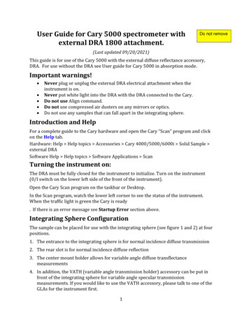
3. Darken the room lights.4. With a thin white card, you should see a green spot at your sample position. (If youcannot see the beam: Block bothsample and reference beams fromentering the integrating sphere. Thenunder the commands menu choosealign to switch the gratings to zeroorder to send white light into theDRA. The white light must notenter the integrating sphere, or itwill damage it!!)5. Check that the beam hits the centerof the M3 mirror and goes throughthe center of L2 and hits the center ofyour sample.6. Most of the mirrors have two knobs,which you can rotate to adjust thevertical and horizontal positions ofthe beam.7. If your sample will be at thereflectance port, use mirror M1 toFigure 2 Photo of diffuse reflectance accessory with beammake the light beam go through thepath.center of the entrance to the sphere,then use M3 to make the beam hityour sample. Redo this several times until the beam does both at once.8. If your sample will be at the transmittance port, use mirror M1 to make the light gothrough the center of M3 and lens L2, then use M3 to hit your sample. Redo do thisseveral times until the beam does both at once.9. Check that the sample beam does not overfill your sample or hit any white surfaces.If the sample is small you need to mask the sample and/or use an aperture torestrict the entrance to the integrating sphere (look in the drawers for the Cary forapertures). You can also reduce the slit height in the software or close theiris/aperture in the sample compartment (Figure 1 & 2). Do not put anything thatcan scatter light close to the beam path at the entrance or exit to the sphere. Thisincludes edges of glass slides.10. If you have very small samples, see the small sample kit in the Users Guide below formore suggestions on small samples11. Check that the reference beam hits mirrors M4 and M5 close to the center and goesthrough the center of L1 and is not clipped at the entrance of the reference beaminto the integrating sphere. Use mirror M5 to center it on the entrance.12. Do not adjust the mirrors with no knobs. If they need adjustment call the GLA,usually they do not need adjustmentRunning your Sample1. Select Setup Instrument Settings Cary Options3
a. Set the wavelength range, and the Y mode, %T, Abs, or %Rb. Set the Ave time (time/data point) as 0.1 s and a Data interval of 1 nm if yourmeasurements will show significant changes (if you have small intensities orsmall changes, you may consider using an Ave time of 0.5 or 1 and a Data intervalof 2 nm/point.c. Under Advanced Settings set SBW, to 2 nm, and Detector and Grating changewavelengths. (Again, if you signals are small you can set the SBW to 4 nm, but itwill increase the beam width and may overfill you sample).d. Under Baseline tab: chose zero/baseline correctione. Under File Storage tab: set whether it prompts to save the spectrum.f. Then click Ok to close the Instrument Settings window.g. Note that the signal to noise ratio, S/N, is a function of the amount of light thatreaches the detector. Increasing the SBW by a factor of 2 will increase the light tothe detector by 4. Decreasing the slight height to reduced will decrease the lightby 4. Increase the Abe time by a factor of 2 will decrease S/N by 2. A setting ofSBW 4 nm and reduced slight height give an approximately square spot on thesample.2. Check that all exits of the integrating sphere are blocked with full reflectors.3. You need to run the 100% Baseline correction with everything in the beam pathexcept your sample. If using an aperture for reflection or transmissionmeasurements, please see the “Aperture kit for small samples” in the User Guidebelow.4. Choose Baseline and run 100% T (or R) scan, then block the sample beam at theentrance to the integrating sphere for the 0% scan.5. It is good practice to run a spectrum with no sample after running Baseline to makesure that you have a good 100% T line.6. Note that the signal to noise (S/N)of your sample spectrum can be no better thanthe S/N of your baselines and will likely be worse by a factor of about1.4 to 2.7. Mount your sample8. Choose Start to run the spectrum9. If you have small intensities (low % R or T) use longer time/point andSBW settings to reduce noise. However, if you increase SBW youStartincrease the light beam size and so need to check if the beam overfillsyour sample.10. Notes:a. The S/N will increase if the SBW is increased, if the slit height is set to full, orif the Ave time (time/point) is increased.b. The time to run the spectra will decrease if the Ave time is decrease or if theData interval is increase.c. Since the SBW setting in the IR is not used and the instrument uses theenergy mode the S/N in the IR is usually very good.4
ToolBarSmall Sample ConsiderationsMost typical lab samples are smaller in size than what the instrument was designed tomeasure. For all three types of measurements (T, C, and R), it is best to under fill thesample so that no light goes around the sample.Spot size - There are two ways of reducing the beam spot size:1. In the Setup: options tab, change the slit width and heighta. Slit width: You can narrow the slit width by changing the SBW parameter.b. Slit height: Under slit height, switch to Reduced. It takes about a minute forthe slit to change.2. Small spot kit (SSK): There are a series of lenses and a mirror that can be put inthe optical path to focus the beam into a smaller spot on the sample. The largemirror (M3) must be changed to the SSK mirror. The SSK mirror is always keptin the T position. There are three lenses (L2, Figure 1) with different focallengths and marked T, C, and R for the three positions of the integrating sphere.3. There are aperture kits that can used with the SSK to adapt a small sampleto the beama. Transmission measurements Aperture kit : There are apertures in thedrawer for the Cary used for transmission measurements. They can be usedon the entrance slit with the white spectralon facing toward the integratingsphere. You ideally would like the sample to completely fill the hole in theaperture and the sample light beam to be about the same size as the aperture.If the sample is smaller than the hole in the aperture you need to mask thesample with black tape.b. Reflection measurements Aperture kit : For normal incidence reflectionmeasurements, the port at the rear of the integration sphere is several inchesin diameter. A series of apertures can be used, which have the whiteSpectralon material on the side that faces toward light beam. The springloaded mount that holds the sample against the integrating sphere needs to be5
taken off. Slide on the appropriate aperture (you can use a little tape to hold itin place) then put the spring-loaded sample mount back on.It is best if the beam spot does not overfill the aperture. If the beam overfillsthe aperture, you can reduce the beam size as mentioned in 1 above or byusing an aperture on the entrance to the integrating sphere or closing theaperture/iris S1 (Figure 1 & 2). If the beam spot overfills the aperture a little,you can correct for this “stray light” by performing a Zero/baselineCorrection. Normally, the 0%T Baseline scan is run by blocking the beambefore it enters the integrating sphere, which accounts for electronic noise.To correct for slight overfilling, do not block the beam and if doing reflectanceleave the exit port open (but with the aperture in place) so that the 0%TBaseline will see light that hits the aperture). This is only useful if therefection from the sample is significantly stronger then the light that hits theexit aperture. One can check the amount of light hitting the apperature byruning a spectrum with the sample light blocked at the entrence slit. It is bestif you can control the beam size so that only the sample is illuminated.Performing a Zero/Baseline Correction: Select this option zero/baselinecorrection, to apply both a 100%T baseline correction and a zero-line correction tothe sample scan. This correction is performed with the raw transmission data and isgiven by:𝑅! 𝑅"% %&'()*'𝑅 ""%, %&'()*' 𝑅"%, %&'()*'Where RS, R0%Baseline, and R100%Baseline are the ratios of the light intensity coming in thesample port to that coming in the reference port for than there is a sample, thesample beam is blocked and when there is no sample, respectively. With this option,the Cary will prompt you to perform a 100%TBaseline first, followed by a0%TBaseline when you perform a baseline collection.Basics of measurement configurationThe wavelength range possible is from 250 to 1800 nm. Scans normally go from long toshort wavelengths. There are two detectors, a PMT and an InGaAs. The wavelength atwhich the system changes from one to the other (accompanied by a grating change) canbe adjusted. Usually, 800 50 nm is a good value for this change over. You can see thechange in the spectrum when you take a baseline (% Transmission or Reflection). Ifyou see a step in the spectrum, it may mean your baseline is bad or that your samplehas a polarization dependency.Setup – The setup button located in the upper left-hand corner defines the scanparameters. The following useful tabs can be found under Setup.Instrument Setting: Cary Options: Here you can set the Wavelength Range, the xand y axes units (nm, cm-1, etc. and A, %T, %R, etc.), as well as the axes ranges.Under scan controls, the average time per data point and the data interval can beset. Note that the Scan Rate will be automatically determined from these values.6
Note if taking a low light spectrum longer time per data point will yield a betterspectrum.Instrument Setting: Advanced Settings: Here you control the Beam Mode,Spectral Band Width (SBW), and Slit Height (see Appendix below for more info). TheDouble beam mode needs to be used for the integrating sphere measurements andthe SBW is typically set to 2 nm.The Slit Height can be used to decrease the beam spot size normally it is set to full.Typically, the UV-Vis button will be selected. If you do not need to go to shorterwavelengths than 400 nm, you can select the Vis button, which will turn off the UVlamp.Instrument Setting: Baseline: Sets the type of baseline(s) corrections used in theScan. The different types of baseline corrections are useful with some accessories.You should collect a zero/baseline correction immediately before scanning a sampleafter the instrument has warmed up for 20 minutes using the same scanparameters that you will use for your sample Also a stored baseline can be used.The Cary WinUV system collects a new baseline when you select any type ofbaseline correction in the Baseline tab of the Setup dialog box and then clickBaseline button in the application window. Depending on the type of correction youhave selected, the Cary will prompt you to a 100%Tbaseline (for the DRA with the100% reference material in the sample positions and, , a 0%Tbaseline (with thesample beam blocked) if a zero/baseline correction was chosen.Once the baselines have been collected, they will be automatically applied to eachcollected sample data point as it is displayed (indicated by the red display). Thecorrection applied is shown below in the Appendix B.A baseline cannot be applied to a sample where the wavelength range of the sampleexceeds that of the baseline. If you change your wavelength range to one outsidethat of the baseline, the Cary will display an error message. Also, the red text in theordinate (y) display, which indicates that the baseline correction mode is activatedwill disappear.See Appendix B for more info on the acquisition, storing, and retrieval of baseline filesInstrument Setting: Independent UV-Vis: This is normally not changed fromdefault Auto in Measurement Mode. In this mode the instrument will collectdouble beam spectra using a fixed SBW in the UV-Vis region and a fixed energy ordetector gain in the NIR region. In this mode, you must set a SBW value for the UVVis region. The normal setting is 2.00 nm. You will find that the gain to the detector(Energy level) will change automatically to maintain the required signal level.You can explicitly set how the instrument controls the detector readings in eachregion. If you want the instrument to scan in another mode i.e., fixe SBE in the NIRor fixed energy (gain) in the UV-Vis region you can set that here, see Appendix A fordetails.7
File Storage: The Auto Store tab allows you to specify if you want to be prompted tostore the collected data. You can store the data in a Batch or Data file at the start orend of a collection. If you set Storage Off you will need to manually store yourunsaved data after the run is complete.Note: In the Scan application, Prompt at Start and Prompt at End saves thespectrum as a data file (*.DSW) unless there are multi or cycle scans beingperformed.Commands In the Menu Bar: Commands can be accessed both from themenu items at the top of the main window and from the application buttons on theright-hand side of the screen. Alternatively, you can use function key shortcuts for someof the commands. These appear next to the item in the Commands menu.Start: Start a Scan using current set up parameters. Function key is F9.Stop: Stop a Scan. If you have selected Storage On in the Auto Store tab, all datacollected is automatically stored in the file specified in the Batch name field of theSave window. Function key is F12.Connect: The Connect command becomes available when more than one softwareapplication is running at any one time. The application that is in use will be onlineand will control the Cary. All other applications will be offline and display theConnect command. If you wish to swap to a different application (and still keepother applications running) you will need to select Connect in the application youwish to connect to the Cary.Zero: Best never to use this. Zeros the current ordinate value using the Startwavelength (or equivalent) value set in the Setup dialog box. Function key is F5. Donot use this if you sample is not zero at this wavelength.Goto: Moves the monochromator to a wavelength specified. Function key is F4. Onlyavailable if the instrument is not currently collecting data.Align: Moves the Cary spectrophotometer to white light (0 nm). Only use if bothsample and reference slits to integrating sphere are blocked. You can then usethis light for aligning accessoriesLamps Off: Switches off all lamps.Lamps On: Switch on selected lamps.Graph menu: The Graph menu allows you to view data in various graphicalformats or in multiple graphs in the Graphics area. You can double-click on the Graphicsarea to toggle the display. The graph functions can also be accessed by clicking one ofthe Toolbar buttons or right-clicking in a graph box or the Graphics area. Not allfunctions are available on every menu.Red Spectrum: The red spectrum in any graph box is the focus spectrum, the onefor which all information appears and the one used for cursor tracking. If you holdthe cursor over a trace, bubble text identifying the trace is shown.8
Trace Preferences: Use to choose the trace(s) to display in the selected spectrum.Graph Preferences: Use to change the appearance of your graph.See Appendix C for more option under the Graph menu as well as the Trace Preferencesand Graph Preferences menusStoring DataUnder the File menu you can save your Method (the Setup configuration used toperform the scan), your Data, or the combination of the Method and Data as a Batch file.File, Save Method As: Used to store the current method. You can store the method,data, report, or graphics template separately or together as a Batch file. The data canalso be saved as a Cary GRAMS file, a comma delimited ASCII spreadsheet file or informats suitable for other Cary software systems (depends on which application youare running).File, Save Data As: Used to store the collected data. You can store the method, data,or report separately or together as a Batch file. The data can also be saved as a CaryGRAMS file, a comma delimited ASCII spreadsheet file or in formats suitable forother Cary software systems (depends on which application you are running). Aftera batch file has been saved, you can use this option to manually save the file as amethod file, a batch file, a comma delimited ASCII spreadsheet file or a Rich TextFormat file.How to Export Collected DataIf you want to export data from a Cary WinUV application into a third-partyapplication, then save your data as an ASCII *.CSV file. To do this:1. Click File Save Data As.2. Click the down arrow next to the Files of type list box.3. Select Spreadsheet ASCII (*.CSV).4. Type your file name into the File name field and click save.How to Combine Data Files into a Batch File:If you have several data files that you need to combine into a batch file, then youneed to:1. Select Open Data.2. . Click the down arrow at the right of the “Files of Type” list box and select'Data' to list all the data files.3. Check the Overlay Data check box.4. Highlight the data files that you require and click Open. The highlighted datafiles will load into the application and appear in the same graph box.5. Select File Save Data As.9
6. A list of previously stored data files will appear. Click the down arrow at theright of the “Files of Type” list box and select 'Batch' to list all the batch files.7. Make sure that the Save only focused trace check box is not checked.8. In the File name field, type in the file name for your new batch file.9. Click Save to create the new batch file. The current method will be stored withthe batch files. All the data files are now combined into the one batch file.Error on Startup1.2.3.4.5.Click ok and let the Cary continue the initialization process.Go to the Commands:GoTo menu option to go to 500 nm.Check that the small aperture in the sample light path is all the way open.Check that there is no sample on any of the ports or inside the integrating sphere.Turn the room lights off. Check that the sample green light beam comes out of thesample monochromator window and goes into the integrating sphere. Check thereference beam in the same way (Figure 2).6. If you don’t see any light coming out of the monochromatora. go back and use the GoTo command again and wait until it completes beforeopening the instrument.b. Check that there is nothing blocking the light from entering integratingsphere.7. Close the sample compartment on the Cary and make sure you hear the interlockclick.8. Turn off the Cary, wait 10 s, and then turn the Cary back on. It should now startupcorrectly.Appendix AHow the Cary 5000/6000i Controls SBW and EnergyIn a spectrometer the intensity observed by the detector changes with wavelength.Double beam spectrometers can monitor the detector readings to make sure that theystay within their optimum region. This can be done in two ways. You can open andclose the slits to increase or decrease the amount of light that reaches the detector, oryou can change the gain on the detector toincrease or decrease the reading. In theformer mode the spectral band width(SBW) will change as the slits open andclose. To prevent changes in the SBW withwavelength the latter method of changingthe gain is used. However, the SBW is inwavelength (nm) units while the spectrumis more linear in energy units (cm-1) soeven with a constant SBW the band width10
in energy will change across the wavelength range (see figure).In the UV-Vis region the detector is a photomultiplier tube (PMT) that allows a largechange in gain with applied voltage. However, in the NIR region, where PbS detectorswere traditionally used this was not possible. Thus, the SBW was normally allowed tovary to maintain the detector output. In the Cary 5000 an InGaAs detector is used thathas very low noise so that an amplifier with settable gain can be used to boost thesignal.In Double or Double Reverse Beam Mode in the UV-Vis region the slit width (SBW) isnormally kept constant, and the gain of the detector is changed. In the NIR region(InGaAs detector) the reverse is normally true i.e. the Energy level is constant and theSBW (slits) changes. Due to the inherent differences between the two types of detector,the different methods of control normally ensure the widest dynamic range and thebest signal to noise. However, in the experimental setup window the mode used can becontrolled in all regions (see below).The instrument uses two detectors (PMT and InGaAs diode), two light sources (W bulband D2 lamp), two gratings in the monochromator, and five order sorting filters. Youcan set the wavelength at which the detectors and gratings change. Both of these aretypically set at 800 nm, if you have an important spectroscopic feature at 800 nm, youcan move the change over 50 nm. The lamp changeover is normally set to 350 nm butagain can be moved 50 nmNote Since gratings are used to disperse the light 2nd (and 3rd ) order light from theoutput beam (i.e., at 800 nm you would also get 400 and 200 nm light) would reach thedetector. The filters changes are at 350, 570, 800, and 1200 nm. You cannot movetheir changeover wavelengths.If collecting data in double beam mode in the UV-Vis regions, you can set how theinstrument controls the detector readings. In SETUP under the independent tab if youchoose how the double beam spectra are collected. With either Auto or Fixed SBW setas the Measurement Mode, you set SBW (slit bandwidth) value in the UV-Vis group.The normal setting is 2.00 nm. You will find that the Energy level will changeautomatically to maintain the required signal level.In double beam mode in the NIR region (where the detector change wavelength occurs,generally l 800nm), in either Auto or Fixed Energy Measurement Mode, the Energylevel is kept constant by changing the slit width (SBW) in the NIR. An Energy setting of1.0 will provide the best signal-to-noise ratio but with a larger SBW. In most cases, therecommended setting is 3.0; this provides a smaller SBW over the entire region and abetter match of the SBW in the NIR region and the Vis region. You will find that the SBWwill change automatically to maintain the required signal level.In double beam mode across the UV-Vis and NIR regions with Fixed SBW set as theMeasurement Mode then you will need to enter values in the SBW fields in both the UVVis and the NIR group boxes. The values can be the same if you want to use the sameSBW across the whole scan or you can set different values for each region, normally theSBW in the NIR is then the SBW in the UV-Vis.11
Note that the SBW is in nm and for a fixed setting of the SBW the resolution in energyterms will be much better in the NIR then in the UV or Vis regions (see figure). Aspectral band width of 2 nm at 400 nm corresponds to 124 cm-1 while at 1200 nm 124cm-1 give a SBW of about 18 nm. This is one reason that most absorption peaks in theNIR are much broader in wavelength then peaks in the UV-Vis regions. It also suggeststhat you can collect at a wider SBW in the NIR than the visible regions.Appendix B:Acquiring, storing, and retrieving baseline filesThe Cary WinUV system collects a new baseline when you select any type of baselinecorrection in the Baseline tab of the Setup dialog box and then click the Baseline buttonin the application window. The then Cary prompts to perform a 100%Tbaseline (withnothing in the beam, or in the case of a Diffuse or Specular Reflectance measurements,with the 100% reference material in position). If required, you are prompted for a0%Tbaseline (the sample beam totally blocked so that the instrument can measure theelectronic zero values).Once collected, they are applied to each collected spectrum. If there is no correspondingdata point in the current baseline, an interpolated point is used. The correction appliedto each point is shown belowA baseline correction cannot be applied if the Y range of the spectra exceeds the 100%baseline. If you change your abscissa range to outside that of the baseline, the Carydisplays an error message and, the red text in the ordinate display which indicates thatbaseline correction mode is activated will disappear.All values within the Baseline abscissa range are corrected, even the value displayedwhile the Cary is idling at a particular wavelength.NoteParameters for Energy, SBW, Beam Mode, Source Changeover, Detector ChangeoverGrating Changeover, Selected Lamp for the collection, Signal-to-Noise Mode, Slit heightand the Independent Control need to be the same in the baseline file and the samplesfiles for a valid correction.Baselines are saved as a part of a batch file. However, if you want, you can also store thebaselines by themselves in a baseline file without the collected data. To do this yousimply select the Baseline (*.CSW) as the Save As Type in the Save As window accessedfrom the File Save Data As menu. When you want to use the baselines for another Scanrun, you simply open the file using either the File Open Data command or click theBaseline button in the Baseline tab of the Setup dialog box.Notesa. If you collect a new baseline, the Cary will use the new baseline in allcorrections. However, the Baseline tab will still display the name of thebaseline in the baseline file. You need to save the collected data as a batch file ifyou want the new baseline included in that file.12
b. All corrections are performed with the raw transmission data that comesdirectly from the instrument. These transmission values are then convertedinto the selected Y mode for display.c. A baseline cannot be applied to a sample where the abscissa range of thesample exceeds that of the baseline. If you wish to use that baseline, then youwill need to reduce the range of the scan by changing the Start and Stop fieldson the Cary tab of the Setup dialog boxTypes of baselines. Choose the type of baseline correction under the Baseline tab inthe Setup menuBaseline Correction: A 100% only baseline correction is applied to the sample scan,𝑅𝑅 ""%./012341Where RS, and R100%Baseline are the ratio of the sample beam to the reference beam withand without the sample.Zero/Baseline Correction: Both a 100%T baseline correction \and a zero-linecorrection is applied to the sample scan.𝑅! 𝑅"% %&'()*'𝑅 ""%, %&'()*' 𝑅"%, %&'()*'With this option, the Cary will prompt you to perform a 100%TBaseline first, followedby a 0%TBaseline when you perform a baseline collection.This baseline option corrects for any inherent variations in the electronic zero line ofthe instrument. Use this baseline option if your samples have areas of very lowtransmission or reflectance as variations in the instrument's zero line will affect yourme
This guide is for use of the Cary 5000 with the diffuse reflectance accessory, DRA. For use without the DRA see User guide for Cary 5000 in absorption mode. Important warnings! Never plug or unplug the external DRA attachment when the instrument is on. Do not put white light into the DRA with the DRA connected to the Cary.