WIXLIB

Unit 22: SamplingDistributionsSummary of VideoIf we know an entire population, then we can compute population parameters such as thepopulation mean or standard deviation. However, we generally don’t have access to datafrom the entire population and must base our information about a population on a sample.From samples, we compute statistics such as sample means or sample standard deviations.However, if we resample, chances are good that we won’t get the same results.This video begins with a population of heights from students in a third grade class at MonicaRos School. A graphic display of the population distribution of heights shows a roughly normalshape with a mean µ 53.4 inches and standard deviation σ 1.8 inches (See Figure 22.1.).Figure 22.1. Population distribution of heights from third-grade class.Next, we draw random samples of size four from the class and record the heights. Figure 22.2shows the results from five samples along with their sample means, which can be found inTable 22.1. Notice that the sample means vary from sample to sample, except for Samples 3and 4 where the sample means match even though the data values differ.Unit 22: Sampling Distributions Student Guide Page 1

Sample1234550515253Height54555657Figure 22.2. Random samples of size four.We can keep sampling until we’ve selected all samples of size four from this population of20 students. If we plot the sample means of all possible samples of size four, we get what iscalled the sampling distribution of the sample mean (See bottom graph in Figure 22.3.).Sample12345Mean, x53.0052.2552.7552.7553.25Table 22.1.Sample means.Figure 22.3. Sampling distribution of the sample mean.Now, compare the sampling distribution of x to the population distribution. Notice thatboth distributions are approximately normal with mean 53.4 inches. However, the samplingdistribution of x is not as spread out as the population distribution.We can calculate the standard deviation of x as follows:Unit 22: Sampling Distributions Student Guide Page 2

σx σn1.8 inchesσx 0.9 inch4Next, we put what we have learned about the sampling distribution of the sample mean touse in the context of manufacturing circuit boards. Although the scene depicted in the video isone that you don’t see much anymore in the United States, we can still explore how statisticscan be used to help control quality in manufacturing. A key part of the manufacturing processof circuit boards is when the components on the board are connected together by passingit through a bath of molten solder. After boards have passed through the soldering bath, aninspector randomly selects boards for a quality check. A score of 100 is the standard, but thereis variation in the scores. The goal of the quality control process is to detect if this variationstarts drifting out of the acceptable range, which would suggest that there is a problem withthe soldering bath.Based on historical data collected when the soldering process was in control, the qualityscores have a normal distribution with mean 100 and standard deviation 4. The inspector’srandom sampling of boards consists of samples of size five. Hence, the sampling distributionof x is normal with a mean of 100 and standard deviation of 4 / 5 1.79 . The inspector usesthis information to make an x control chart, a plot of the values of x against time. A normalcurve showing the sampling distribution of x has been added to the side of the control chart.Recall from the 68-95-99.7% rule, that we expect 99.7% of the scores to be within threestandard deviations of the mean. So, we have added control limits that are three standarddeviations (3 1.79 or 5.37 units) on either side of the mean (See Figure 22.4.). A point outsideeither of the control limits is evidence that the process has become more variable, or that itsmean has shifted – in other words, that it’s gone out of control. As soon as an inspector sees apoint such as the one outside the upper control limit in Figure 22.4, it’s a signal to ask, what’sgone wrong? (For more information on control charts, see Unit 23, Control Charts.)Unit 22: Sampling Distributions Student Guide Page 3

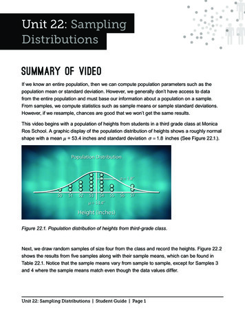
Figure 22.4. Control chart with control limits.So far we’ve been looking at population distributions that follow a roughly normal curve. Next,we look at a distribution of lengths of calls coming into the Mayor’s 24 Hour Hotline call centerin Boston, Massachusetts. Most calls are relatively brief but a few last a very long time. Theshape of the call-length distribution is skewed to the right as shown in Figure 22.5.Figure 22.5. Duration of calls to a call center.To gain insight into the sampling distribution of the sample mean, x , for samples of size 10,we randomly selected 40 samples of size 10 and made a histogram of the sample means.We repeated this process for samples of size 20 and then again for samples of size 60. Thehistograms of the sample means appear in Figure 22.6.Unit 22: Sampling Distributions Student Guide Page 4

Figure 22.6. Histograms of sample means from samples of size 10, 20, and 60.Now let’s compare our sampling distributions (Figure 22.6) with the population distribution(Figure 22.5). Notice that the spread of all the sampling distributions is smaller than the spreadof the population distribution. Furthermore, as the sample size n increases, the spread of thesampling distributions decreases and their shape becomes more symmetric. By the timen 60, the sampling distribution appears approximately normally distributed. What we haveuncovered here is one of the most powerful tools statisticians possess, called the Central LimitTheorem. This states that, regardless of the shape of the population, the sampling distributionof the sample mean will be approximately normal if the sample size is sufficiently large. It isbecause of the Central Limit Theorem that statisticians can generalize from sample data to thelarger population. We will be seeing applications of the Central Limit Theorem in later units onconfidence intervals and significance tests.Unit 22: Sampling Distributions Student Guide Page 5

Student Learning ObjectivesA. Recognize that there is variability due to sampling. Repeated random samples from thesame population will give variable results.B. Understand the concept of a sampling distribution of a statistic such as a sample mean,sample median, or sample proportion.C. Know that the sampling distributions of some common statistics are approximately normallydistributed; in particular, the sample mean x of a simple random sample drawn from a normalpopulation has a normal distribution.D. Know that the standard deviation of the sampling distribution of x depends on both thestandard deviation of the population from which the sample was drawn and the sample size n.E. Grasp a key concept of statistical process control: Monitor the process rather than examineall of the products; all processes have variation; we want to distinguish the natural variation ofthe process from the added variation that shows that the process has been disturbed.F. Make an x control chart. Use the 68-95-99.7% rule and the sampling distribution of x tohelp identify if a process is out of control.G. Be familiar with the Central Limit Theorem: the sample mean x of a large number ofobservations has an approximately normal distribution even when the distribution of individualobservations is not normal.Unit 22: Sampling Distributions Student Guide Page 6

Content OverviewThe idea of a sampling distribution, in general, and specifically about the sampling distributionof the sample mean x , underlies much of introductory statistical inference. The applicationto x charts is important in practice and the discussion of x charts, along with other types ofcontrol charts, continues in Unit 23, Control Charts.If repeated random samples are chosen from the same population, the values of samplestatistics such as x will vary from sample to sample. This variation follows a regular patternin the long run; the sampling distribution is the distribution of values of the statistic in a verylarge number of samples. For example, suppose we start with data from the populationdistribution shown in Figure 22.7. This population is skewed to the right, and clearly notnormally distributed.0510xX152025Figure 22.7. Population distribution.Now, we draw a random sample of size 50 from this population and compute two statistics,the mean and the median, and get 20.7 and 19.8, respectively. Next we take another sampleof size 50 and compute the mean and median for that sample. We keep resampling until wehave a total of 1000 samples. Histograms of the 1000 means and 1000 medians from thosesamples appear in Figures 22.8 and 22.9, respectively. In both cases, the sampling distributionof the statistic appears approximately normally distributed. The sampling distribution of thesample mean, x , is centered around 24 and the sampling distribution of the sample median ataround 22.Unit 22: Sampling Distributions Student Guide Page 7

120Frequency10080604020020222426Sample Mean2830Figure 22.8. Distribution of the sample mean from 1000 samples of size 50.100Frequency8060402001618202224Sample Median262830Figure 22.9. Distribution of the sample median from 1000 samples of size 50.Although basic statistics such as the sample mean, sample median and sample standarddeviation all have sampling distributions, the remainder of this unit will focus on the samplingdistribution of the sample mean, x . If x is the mean of a simple random sample of size n froma population with mean µ and standard deviation σ, then the mean and standard deviation ofthe sampling distribution of x are:µx µσx σnUnit 22: Sampling Distributions Student Guide Page 8

If a population has the normal distribution with mean µ and standard deviation σ, then thesample mean x of n independent observations has a normal distribution with mean µ andstandard deviation σ n . In our example above, the population distribution was not normal(see Figure 22.7). In such cases, the Central Limit Theorem comes to the rescue – if thesample size is large (say n 30), the sampling distribution of x is approximately normal forany population with finite standard deviation.Control charts for the sample mean x provide an immediate application for the samplingdistribution of x . In the 1920’s Walter Shewhart of Bell Laboratories noticed that productionworkers were readjusting their machines in response to every variation in the product. If thediameter of a shaft, for example, was a bit small, the machine was adjusted to cut a largerdiameter. When the next shaft was a bit large, the machine was adjusted to cut smaller. Anyprocess has some variation, so this constant adjustment did nothing except increase variation.Shewhart wanted to give workers a way to distinguish between the natural variation in theprocess and the extraordinary variation that shows that the process has been disturbed andhence, actually requires adjustment.The result was the Shewhart x control chart. The basic idea is that the distribution of samplemean x is close to normal if either the sample size is large or individual measurements arenormally distributed. So, almost all the x -values lie within 3 standard deviations of the mean.The correct standard deviation here is the standard deviation of x , which is σ n (where σ isthe standard deviation of individual measurements). So, the control limits µ 3σ n containthe range in which sample means can be expected to vary if the process remains stable. Thecontrol limits distinguish natural variation from excessive variation.Unit 22: Sampling Distributions Student Guide Page 9