Transcription
Bootstrap Methods andPermutation Tests*wavebreakmedia/Shutterstock16IntroductionThe continuing revolution in computing is having a dramatic influence onstatistics. The exploratory analysis of data is becoming easier as more graphsand calculations are automated. The statistical study of very large and verycomplex data sets is now feasible. Another impact of this fast and inexpensivecomputing is less obvious: new methods apply previously unthinkable amountsof computation to produce confidence intervals and tests of significance insettings that don’t meet the conditions for safe application of the usual methodsof inference.Consider the commonly used t procedures for inference about means(Chapter 7) and for relationships between quantitative variables (Chapter 10).All these methods rest on the use of Normal distributions for data. While nodata are exactly Normal, the t procedures are useful in practice because they*The original version of this chapter was written by Tim Hesterberg, David S. Moore, ShaunMonaghan, Ashley Clipson, and Rachel Epstein, with support from the National ScienceFoundation under grant DMI-0078706. Revisions have been made by Bruce A. Craig and GeorgeP. McCabe. Special thanks to Bob Thurman, Richard Heiberger, Laura Chihara, Tom Moore,and Gudmund Iversen for helpful comments on an earlier version.16.1 The Bootstrap Idea16.2 First Steps in Usingthe Bootstrap16.3 How AccurateIs a BootstrapDistribution?16.4 BootstrapConfidenceIntervals16.5 Significance TestingUsing PermutationTests16-1
16-2Chapter 16 Bootstrap Methods and Permutation TestsLOOK BACKrobust,p. 423testing theequality ofspread,p. 665LOOK BACKvoluntaryresponsesample,p. 190confounding,p. 150are robust. Nonetheless, we cannot use t confidence intervals and tests if thedata are strongly skewed, unless our samples are quite large.Other procedures cannot be used on non-Normal data even when thesamples are large. For example, inference about spread based on Normaldistributions is not robust and, therefore, is of little use in practice.Finally, what should we do if we are interested in, say, a ratio of means,such as the ratio of average men’s salary to average women’s salary? There isno simple traditional inference method for this setting.The methods of this chapter—bootstrap confidence intervals and permuta tion tests—apply the power of the computer to relax some of the conditionsneeded for traditional inference and to do inference in new settings. The bigideas of statistical inference remain the same. The fundamental reasoning isstill based on asking, “What would happen if we applied this method manytimes?’’ Answers to this question are still given by confidence levels andP-values based on the sampling distributions of statistics.The most important requirement for trustworthy conclusions about apopulation is still that our data can be regarded as random samples from thepopulation—not even the computer can rescue voluntary response samples orconfounded experiments. But the new methods set us free from the need forNormal data or large samples. They work the same way for many different sta tistics in many different settings. They can, with sufficient computing power,give results that are more accurate than those from traditional methods.Bootstrap intervals and permutation tests are conceptually simple becausethey appeal directly to the basis of all inference: the sampling distributionthat shows what would happen if we took very many samples under the sameconditions. The new methods do have limitations, some of which we willillustrate. But their effectiveness and range of use are so great that they arenow widely used in a variety of settings.SoftwareBootstrapping and permutation tests are feasible in practice only with soft ware that automates the heavy computation that these methods require. If youare sufficiently expert, you can program at least the basic methods yourself.It is easier to use software that offers bootstrap intervals and permutationtests preprogrammed, just as most software offers the various t intervals andtests. You can expect the new methods to become more common in standardstatistical software.This chapter primarily uses R, the software choice of many statisticiansdoing research on resampling methods.1 There are several packages of func tions for resampling in R. We will focus on the boot package, which offersthe most capabilities. Unlike software such as Minitab and SPSS, R is notmenu driven and requires command line requests to load data and accessvarious functions. All commmands used in this chapter are available on thetext website.JMP, SPSS, and SAS also offer preprogrammed bootstrap and permuta tion methods. JMP offers single-click bootstrapping capabilities to many oftheir tables of results. SPSS has an auxiliary bootstrap module that containsmost of the methods described in this chapter. In SAS, the SURVEYSELECTprocedure can be used to do the necessary resampling. The bootstrap macrocontains most of the confidence interval methods offered by R. You can findlinks for downloading these modules or macros on the text website.
16.1 The Bootstrap Idea16-316.1 The Bootstrap IdeaWhen you completethis section, you willbe able to: Randomly select bootstrap resamples from a small sample usingsoftware or a table of random digits.Find the bootstrap standard error from a collection of resamples.Use computer output to describe the results of a bootstrap analysisof the mean.Here is the example we will use to introduce these methods.EX A M P L E 16.1FACE4Average time looking at a Facebook profile. In Example 12.17 (page 670),we compared the amount of time a Facebook user spends reading differenttypes of profiles. Here, let’s focus on just the average time for the fourthprofile (negative male). Figure 16.1(a) gives a histogram, and Figure 16.1(b)gives the Normal quantile plot of the 21 observations. The data are skewedto the right. Given the relatively small sample size, we have some concernsabout using the t procedures for these data.250.420Times (in minutes)Percent0.30.20.10.015105051015Time (in minutes)(a)2025022210Normal score(b)12FigurE 16.1 (a) The distribution of times (minutes) looking at a negative maleFacebook profile page. (b) Normal quantile plot of the times, Example 16.1.The distribution is right-skewed.The big idea: resampling and the bootstrap distributionLOOK BACKsamplingdistribution,p. 286Statistical inference is based on the sampling distributions of sample sta tistics. A sampling distribution is based on many random samples from thepopulation. The bootstrap is a way of finding the sampling distribution, atleast approximately, from just one sample. Here is the procedure:
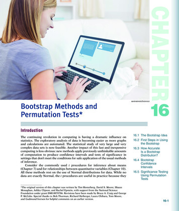
16-4Chapter 16 Bootstrap Methods and Permutation Tests3.77 0.23 5.08 4.35 8.60Mean 4.413.77 0.23 0.23 4.35 4.35Mean 2.593.77 4.35 0.23 8.60 8.60Mean 5.118.60 3.77 0.23 5.08 5.08Mean 4.55FigurE 16.2 The resampling idea. The top box is a sample of size n 5 5 from theFacebook profile viewing time data. The three lower boxes are three resamples from thisoriginal sample. Some values from the original sample are repeated in the resamplesbecause each resample is formed by sampling with replacement. We calculate the statisticof interest, the sample mean in this example, for the original sample and each resample.LOOK BACKresample,p. 424sampling with replacementbootstrap distributionStep 1: Resampling. In Example 16.1, we have just one random sample of21 observations. In place of many samples from the population, create manyresamples by repeatedly sampling with replacement from this one randomsample. Each resample is the same size as the original random sample.Sampling with replacement means that after we randomly draw anobservation from the original sample, we put it back before drawing the nextobservation. Think of drawing a number from a hat and then putting it backbefore drawing again. As a result, any number can be drawn more than once. Ifwe sampled without replacement, we’d get the same set of numbers we startedwith, though in a different order. Figure 16.2 illustrates three resamples froma sample of five observations. In practice, we draw hundreds or thousands ofresamples, not just three.Step 2: Bootstrap distribution. The sampling distribution of a statisticdescribes the values taken by the statistic in all possible samples of the popu lation of the same size. The bootstrap distribution of a statistic summarizesthe values taken by the statistic in all possible resamples of the same size. Thebootstrap distribution gives information (that is, shape and spread) about thesampling distribution.The BOOTsTrAp IdeAThe original sample is representative of the population from which itwas drawn. Thus, resamples from this original sample represent what wewould get if we took many samples from the population. The bootstrapdistribution of a statistic, based on the resamples, represents the samplingdistribution of the statistic.E X A M P L E 16.2FACE4Bootstrap distribution of the mean time looking at a Facebook profile. InExample 16.1, we want to estimate the average time viewing a negativemale Facebook profile, m, so the statistic is the sample mean x. For our onesample of subjects, x 5 7.87 minutes. When we resample, we get differentvalues of x, just as we would if we randomly sampled a new group ofsubjects to survey.We randomly generated 3000 resamples for these data. The mean for theresamples is 7.89 minutes, and the standard deviation is 1.22 minutes. Fig ure 16.3(a) gives a histogram of the bootstrap distribution of the means of3000 resamples from the viewing time data. The Normal density curve with
16-516.1 The Bootstrap IdeaMean time of resamples (in minutes)1246810Mean time of resamples (in minutes)(a)12108623222101Normal score(b)23FigurE 16.3 (a) The bootstrap distribution of 3000 resample means from the sample ofFacebook profile viewing time data. The smooth curve is the Normal density function forthe distribution which matches the mean and standard deviation of the distribution of theresample means. (b) The Normal quantile plot confirms that the bootstrap distribution isslightly skewed to the right but fits the Normal distribution quite well.the mean 7.89, and standard deviation 1.22 is superimposed on the histo gram. A Normal quantile plot is given in Figure 16.3(b). The Normal curvefits the data well, but some skewness is still evident.LOOK BACKcentral limittheorem,p. 298mean andstandarddeviation of x,p. 297bootstrap standard errorAccording to the bootstrap idea, the bootstrap distribution represents thesampling distribution. Let’s compare the bootstrap distribution with what weknow about the sampling distribution.Shape: We see that the bootstrap distribution is nearly Normal. Thecentral limit theorem says that the sampling distribution of the sample meanx is approximately Normal if n is large. So the bootstrap distribution shape isclose to the shape we expect the sampling distribution to have.Center: The bootstrap distribution is centered close to the mean of theoriginal sample, 7.89 minutes versus 7.87 minutes for the original sample.Therefore, the mean of the bootstrap distribution has little bias as an estimatorof the mean of the original sample. We know that the sampling distribution ofx is centered at the population mean m, that is, that x is an unbiased estimateof m. So the resampling distribution behaves (starting from the original sample)as we expect the sampling distribution to behave (starting from the population).Spread: The histogram and density curve in Figure 16.3(a) picture thevariation among the resample means. We can get a numerical measure bycalculating their standard deviation. Because this is the standard deviationof the 3000 values of x that make up the bootstrap distribution, we call it thebootstrap standard error of x. The numerical value is 1.22. In fact, we knowthat the standard deviation of x is syÏn, where s is the standard deviation of
16-6Chapter 16 Bootstrap Methods and Permutation Testsindividual observations in the population. Our usual estimate of this quantityis the standard error of x, syÏn, where s is the standard deviation of our onerandom sample. For these data, s 5 5.65 andsÏnLOOK BACKcentral limittheorem,p. 29855.65Ï215 1.23The bootstrap standard error 1.22 is very close to the theory-based estimate 1.23.In discussing Example 16.2, we took advantage of the fact that statisticaltheory tells us a great deal about the sampling distribution of the sample meanx. We found that the bootstrap distribution created by resampling matchesthe properties of this sampling distribution. The heavy computation neededto produce the bootstrap distribution replaces the heavy theory (central limittheorem, mean, and standard deviation of x) that tells us about the samplingdistribution.The great advantage of the resampling idea is that it often works even whentheory does not apply. Of course, theory also has its advantages: we know ex actly when it works. We don’t know exactly when resampling works, so that“When can I safely bootstrap?’’ is a somewhat subtle issue.Figure 16.4 illustrates the bootstrap idea by comparing three distributions.Figure 16.4(a) shows the idea of the sampling distribution of the sample meanx: take many simple random samples (SRS) from the population, calculate themean x for each sample, and collect these x-values into a distribution.Figure 16.4(b) shows how traditional inference works: statistical theorytells us that if the population has a Normal distribution, then the samplingdistribution of x is also Normal. If the population is not Normal but oursample is large, we can use the central limit theorem. If m and s are themean and standard deviation of the population, the sampling distribution ofx has mean m and standard deviation syÏn. When it is available, theory iswonderful: we know the sampling distribution without the impractical task ofactually taking many samples from the population.SRS of size nx–SRS of size nx–SRS of size nx–······POPULATIONunknown mean Sampling distribution(a)FigurE 16.4 (a) The idea of the sampling distribution of the sample mean x: take verymany samples, collect the x values from each, and look at the distribution of these values.(b) The theory shortcut: if we know that the population values follow a Normal distribution,theory tells us that the sampling distribution of x is also Normal. (c) The bootstrap idea: whentheory fails and we can afford only one sample, that sample stands in for the population, / nand the distribution of x in many resamplesstands in for the sampling distribution. Theory
Sampling distribution(a)16.1 The Bootstrap Idea16-7 / n Theory Sampling distributionNORMAL POPULATIONunknown mean (b)One SRS of size nResample of size nx–Resample of size nx–Resample of size nx–······POPULATIONunknown mean Bootstrap distribution(c)FigurE 16.4 (Continued)Figure 16.4(c) shows the bootstrap idea: we avoid the task of taking many sam ples from the population by instead taking many resamples from a single sample.The values of x from these resamples form the bootstrap distribution. We use thebootstrap distribution rather than theory to learn about the sampling distribution.uSE Your KnoWLEdgE16.1 A small bootstrap example. To illustrate the bootstrap procedure,let’s bootstrap a small random subset of the Facebook profile data:4.02FACE463.034.358.331.405.08(a) Sample with replacement from this initial simple random sample(SRS) by rolling a die. Rolling a 1 means select the first member of theSRS, a 2 means select the second member, and so on. (You can alsouse Table B of random digits, responding only to digits 1 to 6.) Create20 resamples of size n 5 6.(b) Calculate the sample mean for each of the resamples.(c) Make a stemplot of the means of the 20 resamples. This is thebootstrap distribution.(d) Calculate the bootstrap standard error.
16-8Chapter 16 Bootstrap Methods and Permutation Tests16.2 Standard deviation versus standard error. Explain the differencebetween the standard deviation of a sample and the standard error ofa statistic such as the sample mean.Thinking about the bootstrap ideaIt might appear that resampling creates new data out of nothing. This seemssuspicious. Even the name “bootstrap’’ comes from the impossible image of“pulling yourself up by your own bootstraps.’’2 But the resampled observationsare not used as if they were new data. The bootstrap distribution of theresample means is used only to estimate how the sample mean of one actualsample of size 21 would vary because of random sampling.Using the same data for two purposes—to estimate a parameter and also toestimate the variability of the estimate—is perfectly legitimate. We do exactlythis when we calculate x to estimate m and then calculate syÏn from the samedata to estimate the variability of x.What is new? First of all, we don’t rely on the formula syÏn to estimate thestandard deviation of x. Instead, we use the ordinary standard deviation of themany x-values from our many resamples.3 Suppose that we take B resamplesand call the means of these resamples x* to distinguish them from the mean xof the original sample. We would then find the mean and standard deviationof the x*’s in the usual way.To make clear that these are the mean and standard deviation of the meansof the B resamples rather than the mean x and standard deviation s of theoriginal sample, we use a distinct notation:meanboot 5LOOK BACKdescribingdistributionswith numbers,p. 27SEboot 51Bo x*Î1B21o (x* 2 meanboot)2These formulas go all the way back to Chapter 1. Once we have the values x*,we can just ask our software for their mean and standard deviation.Because we will often apply the bootstrap to statistics other than thesample mean, here is the general definition for the bootstrap standard error.BOOTsTrAp sTAndArd errOrThe bootstrap standard error, SEboot, of a statistic is the standarddeviation of the bootstrap distribution of that statistic.Second, we don’t appeal to the central limit theorem or other theory to tellus that a sampling distribution is roughly Normal. We look at the bootstrapdistribution to see if it is roughly Normal (or not). In most cases, the boot strap distribution has approximately the same shape and spread as the sam pling distribution, but it is centered at the original sample statistic valuerather than the parameter value.In summary, the bootstrap allows us to calculate standard errors for sta tistics for which we don’t have formulas and to check Normality of the sam pling distribution of statistics that theory doesn’t easily handle. To apply thebootstrap idea, we must start with a statistic that estimates the parameter we
16.1 The Bootstrap Idea16-9are interested in. We come up with a suitable statistic by appealing to anotherprinciple that we have often applied without thinking about it.The pLug-In prInCIpLeTo estimate a parameter, a quantity that describes the population, use thestatistic that is the corresponding quantity for the sample.The plug-in principle tells us to estimate a population mean m by thesample mean x and a population standard deviation s by the sample standarddeviation s. Estimate a population median by the sample median and apopulation regression line by the least-squares line calculated from a sample.The bootstrap idea itself is a form of the plug-in principle: substitute the datafor the population and then draw samples (resamples) to mimic the processof building a sampling distribution.using softwareSoftware is essential for bootstrapping in practice. Here is an outline of theprogram you would write if your software can choose random samples froma set of data but does not have bootstrap functions:Repeat B times {Draw a resample with replacement from the data.Calculate the resample statistic.Save the resample statistic into a variable.}Make a histogram and Normal quantile plot of the B resample statistics. Calculatethe standard deviation of the B statistics.EX A M P L E 16.3FACE4FigurE 16.5 R output for theFacebook profile viewing timebootstrap, Example 16.3.using software. R has packages that contain various bootstrap functions, sowe do not have to write them ourselves. If the 21 viewing times are savedas a variable, we can use functions to resample from the data, calculate themeans of the resamples, and request both graphs and printed output. Wecan also ask that the bootstrap results be saved for later access.The function plot.boot will generate graphs similar to those in Figure 16.3so you can assess Normality. Figure 16.5 contains the default output from acall of the function boot. The variable Time contains the 21 viewing times, thefunction theta is specified to be the mean, and we request 3000 resamples.ORDINARY NONPARAMETRIC BOOTSTRAPCall:boot(data Time, statistic theta, R 3000)Bootstrap Statistics :originalbiast1*7.8704760.02295317std. error1.216978
16-10Chapter 16 Bootstrap Methods and Permutation TestsThe original entry gives the mean x 5 7.87 of the original sample. Bias is thedifference between the mean of the resample means and the original mean.If we add the entries for bias and original, we get the mean of the resamplemeans, meanboot:7.87 1 0.02 5 7.89The bootstrap standard error is displayed under std. error. All these valuesexcept original will differ a bit if you take another 3000 resamples becauseresamples are drawn at random.SEcTion 16.1 SUMMARy To bootstrap a statistic such as the sample mean, draw hundreds ofresamples with replacement from a single original sample, calculate thestatistic for each resample, and inspect the bootstrap distribution of theresample statistics. A bootstrap distribution approximates the sampling distribution of thestatistic. This is an example of the plug-in principle: use a quantity basedon the sample to approximate a similar quantity from the population. A bootstrap distribution usually has approximately the same shape andspread as the sampling distribution. It is centered at the statistic (from theoriginal sample) while the sampling distribution is centered at the parameter(of the population). Use graphs and numerical summaries to determine whether the bootstrapdistribution is approximately Normal and centered at the original statisticand to assess its spread. The bootstrap standard error is the standarddeviation of the bootstrap distribution. The bootstrap does not replace or add to the original data. We use thebootstrap distribution as a way to estimate the sampling distribution of astatistic based on the original data.SEcTion 16.1 EXERCISESFor Exercises 16.1 and 16.2, see pages 16-7–16-8.16.3 Gosset’s data on double stout sales. WilliamSealy Gosset worked at the Guinness Brewery in Dublinand made substantial contributions to the practice ofstatistics. In Exercise 1.65 (page 48), we examinedGosset’s data on the change in the double stout marketbefore and after World War I (1914–1918). For variousregions in England and Scotland, he calculated the ratioof sales in 1925, after the war, as a percent of sales in1913, before the war. Here are the data for a sample ofsix of the regions in the original data:STOUT6(a) Do you think that these data appear to be from aNormal distribution? Give reasons for your answer.(b) Select five resamples from this set of data.(c) Compute the mean for each resample.16.4 Find the bootstrap standard error. Refer to yourwork in the previous exercise.STOUT6(a) Would you expect the bootstrap standard error to belarger, smaller, or approximately equal to the standarddeviation of the original sample of six regions? Explainyour answer.(b) Find the bootstrap standard error.BristolEnglish PEnglish Agents944678GlasgowLiverpoolScottish661402416.5 Read the output. Figure 16.6 gives a histogramand a Normal quantile plot for 3000 resample meansfrom R. Interpret these plots.
16-11100t*800.0200.0150.000FigurE 16.6 R output for thechange in double stout salesbootstrap, Exercise 16.5.400.005600.010Density0.0251200.03016.1 The Bootstrap Idea2060100t*140–3 –2 –1 0 1 2 3Normal Score(d) The bootstrap distribution is created by resamplingwith replacement from the population.ORDINARY NONPARAMETRIC BOOTSTRAPCall:boot(data stout, statistic theta, R 3000)Bootstrap Statistics :originalbiast1*74.66667 -0.2038889std.error14.90047FigurE 16.7 R output for the change in double stoutsales bootstrap, Exercise 16.6.16.6 Read the output. Figure 16.7 gives output from Rfor the sample of regions in Exercise 16.3. Summarizethe results of the analysis using this output.Inspecting the bootstrap distribution of a statistic helpsus judge whether the sampling distribution of the sta tistic is close to Normal. Bootstrap the sample mean xfor each of the data sets in Exercises 16.8 through 16.12using 2000 resamples. Construct a histogram and aNormal quantile plot to assess Normality of the boot strap distribution. On the basis of your work, do youexpect the sampling distribution of x to be close to Nor mal? Save your bootstrap results for later analysis.16.8 Bootstrap distribution of average IQ score.The distribution of the 60 IQ test scores in Table 1.1(page 14) is roughly Normal (see Figure 1.7) and thesample size is large enough that we expect a Normalsampling distribution.IQ(b) The bootstrap distribution is created by resamplingwithout replacement from the original sample.16.9 Bootstrap distribution of StubHub! prices. Weexamined the distribution of the 518 tickets for theNational Collegiate Athletic Association (NCAA) Women’sFinal Four Basketball Championship posted for sale onStubHub! on June 28, 2014, in Example 1.48 (page 69).The distribution is clearly not Normal; it has three peakspossibly corresponding to three types of seats. We viewthese data as coming from a process that gives seat pricesfor an event such as this.STUB1(c) When generating the resamples, it is best to use asample size smaller than the size of the original sample.16.10 Bootstrap distribution of time spent watchingtraditional television. The hours per week spent watching16.7 What’s wrong? Explain what is wrong with each ofthe following statements.(a) The standard deviation of the bootstrap distributionwill be approximately the same as the standard deviationof the original sample.
16-12Chapter 16 Bootstrap Methods and Permutation Teststraditional television in a random sample of eight full-timeU.S. college students (Example 7.1, page 411) are3.016.5 10.540.55.533.50.06.5The distribution has no outliers, but we cannot comfortablyassess Normality from such a small sample.TVTIME16.11 Bootstrap distribution of Titanic passengerages. In Example 1.36 (page 52), we examined thedistribution of the ages of the passengers on the Titanic.There is a single mode around 25, a short left tail, and along right tail. We view these data as coming from aprocess that would generate similar data.TITANIC16.12 Bootstrap distribution of average audio filelength. The lengths (in seconds) of audio files found on aniPod (Table 7.5, page 470) are skewed. We previouslytransformed the data prior to using t procedures.SONGSuse it to find the standard error syÏn of the sample mean.How closely does your result agree with the bootstrapstandard error from your resampling in Exercise 16.10?16.14 Service center call lengths. Table 1.2 (page 17)gives the service center call lengths for a sample of 80calls. See Example 1.15 (page 15) for more details aboutthese data.CALLS80(a) Make a histogram of the call lengths. The distributionis strongly skewed.(b) The central limit theorem says that the samplingdistribution of the sample mean x becomes Normal as thesample size increases. Is the sampling distribution roughlyNormal for n 5 80? To find out, bootstrap these data using1000 resamples and inspect the bootstrap distribution ofthe mean. The central part of the distribution is close toNormal. In what way do the tails depart from Normality?16.13 Standard error versus the bootstrap standarderror. We have two ways to estimate the standarddeviation of a sample mean x: use the formula syÏn forthe standard error, or use the bootstrap standard error.16.15 More on service center call lengths. Here is anSRS of 10 of the service center call lengths from Exercise16.14:CALLS10(a) Find the sample standard deviation s for the 60 IQtest scores in Exercise 16.8 and use it to find the standarderror syÏn of the sample mean. How closely does yourresult agree with the bootstrap standard error from yourresampling in Exercise 16.8?We expect the sampling distribution of x to be less closeto Normal for samples of size 10 than for samples of size80 from a skewed distribution.(b) Find the sample standard deviation s for theStubHub! ticket price data in Exercise 16.9 and use it tofind the standard error syÏn of the sample mean. Howclosely does your result agree with the bootstrap standarderror from your resampling in Exercise 16.9?(c) Find the sample standard deviation s for the eighttraditional television viewing times in Exercise 16.10 and104102352115632567917959(a) Create and inspect the bootstrap distribution ofthe sample mean for these data using 1000 resamples.Compared with your distribution from the previousexercise, is this distribution closer to or farther awayfrom Normal?(b) Compare the bootstrap standard errors for your twosets of resamples. Why is the standard error larger for thesmaller SRS?16.2 First steps in using the BootstrapWhen you completethis section, you willbe able to: Determine when it is appropriate to use the bootstrap standard error andthe t distribution to find a confidence interval.Use the bootstrap standard error and the t distribution to find aconfidence interval.To introduce the key ideas of resampling and bootstrap distributions, westudied an example in which we knew quite a bit about the actual samplingdistribution. We saw that the bootstrap distribution agrees with the samplingdistribution in shape and spread.The center of the bootstrap distribution is
22_Moore_13387_Ch16_01-57.indd 1 07/10/16 3:26 PM Bootstrap Methods and Permutation Tests* Introduction 16.1 The Bootstrap Idea 16.2 First Steps in Using the Bootstrap 16.3 How Accurate Is a Bootstrap Distribution? 16.4 Bootstr ap Confidence In