Transcription
Developing Tools for Analysis of Text DataNovember 2016Randall Powers, Brandon Kopp and Wendy MartinezOffice of Survey Methods Research, U.S. Bureau of Labor StatisticsPowers.Randall@bls.govAbstract: Many surveys at the Bureau of Labor Statistics have unstructured or semi-structured text fields.Most of these sources of text are not analyzed because users usually do not know what types of analysescan be done, and they lack easy-to-use and inexpensive tools to exploit the text data. This paper will describean application that was developed to analyze survey text data.Key words: Survey data; Text data; Text analytics workflow; Software tool development;Statistical learning1. IntroductionText analysis is the process of extracting information from written language, and it is animportant activity for many Bureau of Labor Statistics (BLS) programs. For example, an analystmight read job titles to assign occupation classifications, check websites for the latest product andprice information, or scan news articles to track important economic events.Currently, there are no existing tools at BLS to look at open ended text data from surveyinterviews. Ultimately, we want a tool that will allow us to find themes amongst the interview datausing word clouds and simple visualization, and to be able to export our results to a useful file. Thiskind of analysis can be done in R, but there’s a steep learning curve. We wanted something simplerto use such that the analyst doesn’t have to write his or her own R code. It can be done using SASor SPSS, but those can be expensive, and don’t allow the user control over the tools. We wantedsomething that we ourselves designed and customized.Shiny is an R package that makes it easy to build interactive web applications straight from R.No knowledge of Javascript or HTML is necessary. All coding is done using R. Additionally, thepackage contains many useful functions and tools that the user would otherwise have to write fromscratch. Hence, the amount of R coding that is actually necessary is greatly decreased. Wedetermined that developing an application using the R Shiny package would best suit our needs.This paper will describe the R Shiny application we developed. Each section will detail aseparate application screen. These screens will include each of these tabbed items displayed inFigure 1.2. The ‘Welcome Screen’ TabWhen the application is run, the Welcome Screen (Figure 2), the first of six tabs, appears bydefault. This screen gives the user information about file formats and within file formatting. Theimported file must be in one of three formats: text-delimited (e.g. .csv, .tsv), Excel, or R (i.e. RDSfile).The data should be formatted so that the text information you are interested in exploring is inone column. Each row of the data should be a unique 'document.' That is, it should make sense asa unit. You might have one row (document) for each respondent to a survey.The Welcome Screen example (see Figure 2a) uses a national parks dataset. Each textdescription of a national park is a text variable to be analyzed (referred to as the “document”), and
Jthe user would have the option to group by various categories such as Region. The user would belooking for common themes among the descriptions of national parks.Once the user has the data ready to go, they can go to the tab marked 'Step 1: Upload YourData.3. The ‘Load Your Data’ TabThis tab enables the user to load their data file from anywhere on their computer. The file mustbe in either Excel, CSV, or R format. Please see Figure 3 for more details.The user can optionally choose to use a stopwords list imported via an Excel file. This is a listof common words that are excluded from the analyses. For example, “the”, “and”, “but”, etc. areoften of little or no use in differentiating one document from another. The text analysis tool, bydefault, removes 175 stopwords, but a user may want to customize this list (or create their own), assome common words may be of use when classifying documents.For demonstration purposes, a respondent burden dataset is used. The Office of SurveyMethods Research at BLS conducted a survey in which respondents were asked a number ofquestions about expenditures and then were asked how burdensome they found the survey. Tobetter understand their burden rating, respondents were asked to list an activity that they find “notat all burdensome”, an activity that they find “somewhat burdensome”, and an activity that theyfind “extremely burdensome”. The open-ended description of activities at these different burdenlevels is what we will use to demonstrate the application.Once the user has loaded his file, they can begin the analysis by clicking on the next tab,‘Exploratory Plots’.4. The ‘Exploratory Plots” TabOn the third tab (shown in Figure 4), the user can look at wordcloud and frequency plots oftheir data. The user first specifies the text variable they wish to analyze. For the burden datasetexample, any of the three comparison burden categories work equally well. In this example, theuser does not need to choose a categorical variable for this set of data.For other datasets, the user can choose a categorical variable to compare text. For example,with the national parks dataset that was on the welcome screen, we might choose geographic regionas our categorical variable.The NGrams slider creates longer word strings; it defaults to single word strings (unigrams),but can be increased to 2-word strings (bigrams), 3-word strings (trigrams), etc. Hence, the usercan specify whether they want to analyze single words, or multiple word phrases. They can alsochoose to exclude certain words. When the user is done choosing their desired specifications, aword cloud and a chart with word frequency or word percentage (not pictured) is produced. Whenthere is a categorical variable, the user can see which text it more prevalent in certain categories,and see the relative frequencies of the most common words in the frequency chart.5. The ‘Context Viewer’ TabThe user may wish to see the context in which a word or phrase was used. When the userchooses this tab (see Figure 5), the user can find a word or phrase in the text containing their searchtext. In the burden example, the user might wish to compare in what ways the word “watching”was used as part of strings for Not At All Burdensome activities.6. The ‘Clustering’ TabThe main feature of the application is the clustering tab (Figure 6). Document clusteringinvolves the use of descriptors and descriptor extraction. The user must specify a few parameters
Jbefore results are produced. This includes choosing the text variable to analyze, the dimensionreduction method, the N-gram size, as well as elimination of stop words and the use of stem words(i.e., truncating words so that base words can be combined). The user can choose to see the resultsas a frequency count, as binary (word present/not present), as the proportion in the document, or asthe inverse document frequency. After the input parameters are specified, a number of results areproduced.These results (see Figures 6a and 6b) include a Document Clustering Plot. Based on the numberof clusters specified, we see n different clusters. Cluster groupings are created using K-nearestneighbors. Here we’re looking for tightly defined clusters so that we can look at their contents andsee what makes them unique. One weakness of the current clustering system in the current textanalysis application is that it compresses hundreds or thousands of terms into just two difficult tointerpret dimensions. This is done for visualization purposes. Two dimensions may be too few toadequately capture the variation between documents. More dimensions will be allowed in futureversions of the application.Another result is a Word Dimension Plot, which shows the distribution of words along our twocompressed dimensions. It can help us interpret the meaning of the two dimensions in the graph.Comparative Word Clouds are also produced. They show the dominant terms in each cluster andwhere terms were more strongly related to a particular cluster. A Top Five Terms per cluster chartis also produced. This lists the five most used terms in each cluster. A Documents Per Cluster tableis also produced. This shows us the number of documents that contain terms in each particularcluster, thus giving the user an idea of how exclusive a cluster is. The more documents that appearin a cluster, the less exclusive. A Latent Semantic Variables Matrix, which s pairwise scatterplotsof multiple dimension. As mentioned earlier, the application currently reduces the dataset to twodimensions for visualization purposes. This plot is an attempt to explore greater dimensionality inthe data and perhaps find a pair of dimensions that creates more well-defined clusters. In a futureversion of the application, users will be able to select which pair of dimensions they want to beused for the primary analysis.7. The ‘Output Data” TabThe Output Data Tab allows the user to output a term document matrix (or document termmatrix) into an Excel or CSV file. Again, the user chooses which text and categorical variables toanalyze. The user can choose to collapse the results for all documents into one row, or have theresults by document. There are also have a number of options that were previously seen on thecluster tab.8. Final CommentsThe application is still currently in the development phase. The authors plan to make theapplication publicly available upon completion.9.ReferencesBouchet-Valat, Milan (2014). SnowballC: Snowball stemmers based on the C libstemmerUTF-8 library. R package version 0.5.1. https://CRAN.R-project.org/package SnowballCChang, Winston, Joe Cheng, JJ Allaire, Yihui Xie and JonathanMcPherson (2016). shiny:Web Application Framework for R. R package version 0.13.1. https://CRAN.Rproject.org/package shiny
Dahl, David B. (2016). xtable: Export Tables to LaTeX or HTML. Rpackage version 1.82. https://CRAN.R-project.org/package xtableDragulescu, Adrian A.(2014). xlsx: Read, write, format Excel 2007 and ps://CRAN.Rproject.org/package xlsxFeinerer, Ingo and Kurt Hornik (2015). tm: Text Mining Package. R package version 0.62. https://CRAN.R-project.org/package tmFellows, Ian (2014). wordcloud: Word Clouds. R package version 2.5. https://CRAN.Rproject.org/package wordcloudMartinez, Wendy and Alex Measure (2013). Statistical Analysis of Text in Survey Records.Presented at Federal Committee on Statistical Methodology Research 5/C3 Martinez 2013FCSM.pdfMeasure, Alex (2016). Bureau of Labor Statistics Text Analysis Team internal document.Musialek, Chris. Philip Resnik and S.Andrew Stavisky (2016) Using Text AnalyticTechniques to Create Efficiencies in Analyzing Qualitative Data: A Comparison betweenTraditional Content Analysis and a Topic Modeling Approach. Presented at AmericanAssociation for Public Opinion Research Conference.R Core Team (2015). foreign: Read Data Stored by Minitab, S, SAS, SPSS, Stata, Systat,Weka, dBase, . R package version 0.8-66. https://CRAN.R-project.org/package foreignR Core Team (2016). R: A language and environment for statistical computing. RFoundation for Statistical Computing, Vienna, Austria.URL http: www.R-project.org/Solka, Jeffrey L. (2007). Text Data Mining: Theory and Methods. Statistics Surveys, 2, 94–112. kham. Hadley (2016). scales: Scale Functions for Visualization. Rpackage version0.4.0. https://CRAN.R-project.org/package scalesWickham, Hadley (2007). Reshaping Data with the reshape Package.Journal of StatisticalSoftware, 21(12), 1-20. URL http://www.jstatsoft.org/v21/i12/.Wickham. Hadley (2015). stringr: Simple, Consistent Wrappers for Common StringOperations. R package version 1.0.0. https://CRAN.R-project.org/package stringrWickham, Hadley and Romain Francois (2015). dplyr: A Grammar of Data Manipulation.R package version 0.4.3. https://CRAN.R-project.org/package dplyrWickham, H. ggplot2: Elegant Graphics for Data Analysis. Springer-Verlag New York,2009.Wild, Fridolin (2015). lsa: Latent Semantic Analysis. R package version 0.73.1.https://CRAN.R-project.org/package lsaXie, Yihui(2015). DT: A Wrapper of the JavaScript Library 'DataTables'. R packageversion 0.1. https://CRAN.R-project.org/package DT
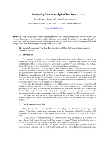
Figure 1: Application TabsFigure 2: The ‘Welcome Screen’ Tab
Figure 2a: The ‘Welcome Screen’ Tab (Example)
Figure 3: The Load Data Tab
Figure 4: The ‘Exploratory Plots” Tab (with output)
Figure 4a: The ‘Exploratory Plots” Tab (with output, #2)
Figure 5: Context Viewer Tab (output)
Figure 6: The ‘Clustering’ Tab
Figure 6a: The ‘Clustering’ Tab (output #1)Figure 6b: The ‘Clustering’ Tab (output #2)
Figure 7: The ‘Output’ Tab
an application that was developed to analyze survey text data. Key words: Survey data; Text data; Text analytics workflow; Software tool development; Statistical learning . 1. Introduction. Text analysis is the process of extracting information from written language, and it is an important activity for many Bureau of Labor Statistics (BLS .