Transcription
APPLICATION OF LESLIE MATRIX MODELSTO WILD TURKEY POPULATIONSby Wen-Ching LiNorth Carolina State UniversityDepartment of StatisticsBiomathematics Graduate ProgramRaleigh1994
CONTENTSABSTRACT1THE LESLIE MATRIX MODEL2Introduction2Model structure2Parameter estimation7Eigensystem9Stable age distribution11Application and generalization14APPLICATION TO EASTERN WILD TURKEY IN lOWA16Introduction16Objectives17Model structure17Parameter estimation20Result and discussion23Future work36
ABSTRACTThe Leslie matrix model is a popular and useful method for population projection based onage specific survival and fecundity rates.The first part of this project will describe thetheorems, properties, application, and development of the Leslie matrix model in detail. In thesecond part, specific Leslie models are developed for wild turkeys in Iowa.The Leslie matrix model has become very popular because of its easy understanding bybiologists and because many theoretical properties can be easily studied using matrix algebra.In the example for Iowa wild turkey populations, a simple, linear, deterministic model basedon the Leslie model is built. The model's simplicity makes it easy to understand and analyze.However, its simplicity also means that it is far from biological reality. There are too fewparameters to adequately describe the complexity of a real turkey population. However, it isa good model on which to build more complex and realistic models which may allowstochasticity and density dependence of survival and fecundity rates.1
THE LESLIE MATRIX MODELIntroductionBirths and deaths are age-dependent in most species except very simple organisms. It isusually necessary to take account of a population's age structure to get a reliable description ofits dynamics. The English biologist P .R.Leslie (1945) introduced a model which uses the agespecific rates of fertility and mortality of a population. He developed the model based on theuse of matrices. The matrix form makes the model flexible and mathematically easy to study.This basic model is an increasingly popular tool for describing population dynamics of plants(Usher 1969) and animals (Yu 1990, Crouse 1987). The Leslie matrix model is widely used toproject the present state of a population into the future, either as an attempt to forecast the agedistribution, or as a way to evaluate life history hypotheses by considering different sets ofsurvival and fecundity parameters.Model structureIn the simplest Leslie matrix model (Leslie 1945), only females are considered. The femalepopulation can be divided into several categories by age or by size. The classification styles andtheir differences will be discussed later in this section.If it's grouped by age, the groupintervals are supposed to have equal length of time. For example, it may be 5 years for humanand 2 years for large whales (Cullen 1985). We assume that the survival and fecundity rates2
of each category are constant over time and therefore not dependent on population density.Definenj(t) the number of females alive in the group i at time t,Pj the probability that a female of group i at time t will be alive in group i 1 at time t 1,(t 1 means t one unit of time), Pi lies between 0 and 1,F j the number of daughters born per female in group i from time t to time t 1,let i 1,2, . ,x, thennl(t l) F1*n](t) F 2 *n 2(t) . Fx*nx(t)n2 (t l) P1*n)(t)n2(t 1) P 2 *n2(t)(1.1)These equations can be represented in matrix form as(1.2)n(t 1) A n(t)where n(t) is a column vector with components of the number of individuals in each recognizedcategory at time t.A is a nonnegative, square matrix of order x with all the elements zeroexcept those in the first row and in the subdiagonal immediately below the principal diagonal.3
A FiF2 F3P1aaaP2 00 P3a000FX - 1 FxaaaaaaPX - 10(1.3)A is known as the "Leslie matrix" based on age classifications or the "population projectionmatrix" modeled on stage classifications (Lefkovitch 1965, Groenendaeo et al. 1988, Crouse etal. 1987).The projection matrix was introduced by Lefkovitch (1965).projection matrix model are not necessarily related to age.The stages in theIts main assumption is that allindividuals in a given stage are subject to identical mortality, growth, and fecundity schedules.These matrices are more complicated in appearance than the Leslie matrices, but have almostthe same analytical method.Fig. 1.1 shows the life cycle graph depending on differentdecomposition of the life cycle.The arrows in the graph indicate the transitions which are possible for an individual fromone time to the next. The Leslie matrix corresponding with the life cycle graph (A) in Fig 1.1is just the same as (1.3) and much simpler than the projection matrix for the stage-classifiedpopulation, (8) of Fig 1.1, obtained as follows:4
.F u F 12 F13 F 14P 21 P 22 P 23A.00,0PX - 100J,Age class Pl1 x-lx-lPX - 1xPx xFxF2,-Age classlF llJ,StagePX PxP22, .l -.JP21 .xFixP32Stager--,Age classPx-1F l2;1x-211B.(1. 4)00F,,/0P 32 P 33 P 340AF 1XI.2.,P23IJ'.StageP xx-1J .Px-1 xrx Fig 1.1 Life cycle graphs for two choices of categories. (A) Age-classified population. (B)One example of stage-classified population.5
In the stage-classified model, the possibility of an individual of group i moving backwards to theprevious group, moving forwards to the next group, or staying the same group at next timeperiod is considered.The choice of categories is a very important step in establishing a population matrix model(Groenendael et al. 1988). Since sometimes it is hard to determine age-specific parameters ofthe model for some organisms with variable development, stage categories may be moreappropriate than age categories (e.g. for turtles, Crouse 1987).For other organisms likemammals and birds, their development is more dependent on age than size and therefore agecategories are used frequently.If age and size are both important and significant interactions exist between them, a twodimensional model using both stages and age classes simultaneously can be developed(Yu 1990).In Yu' s study, developmental stages are as meaningful as chronological age classes in the cornearworm (CEW) management.He divided the CEW population into five stages and split thefirst stage into four age groups, the remaining stages into six age groups, except taking the laststage as a single age group. Thus, his projection matrix is a 23*23 matrix taking both stage andage into account.In this project, I will mainly discuss the properties of an age-classified matrix model basedon form (1.3). The model has linear, time invariant functions which project the current stateof the population into the next state. The female population alone will be considered.6
Parameter estimationSurvival probability PiThe values of Pi can be obtained from a life table or experimental data.It is usuallyassumed that (Leslie 1945, Poole 1974)L 1p . i- - (1.5)L· where L i the number alive in the age group i to i 1 in the stationary or life table agedistribution. Pi is assumed to be constant over a unit of time and not dependent on the totalnumber in the population. Actually, seasonal differences and density dependence of the survivalrate do exist, but we assume that they are not significant enough to count.Fecundity rates F jF; is determined not only by the average number of female births per mother per timeperiod, m j in the life table, but also by infant survival rates (Leslie 1945, Groenendael et al.1988). Populations can be divided into two cases of breeding systems, 'birth-flow' populationwith continuous reproduction and 'birth-pulse' populations with discrete reproduction (Caughley1977).Populations, e.g. human, of the first case produce offspring at a rate almost constantthroughout the year and those of the second case produce offspring over a restricted season, e.g.7
blue whale. In birth-flow populations, the estimation of F i involves integration of continuousfertility and infant mortality functions over the time interval (Leslie 1945).For birth pulse populations reproduction is during a short period of time per year.It isimportant to know the exact breeding period with respect to the time step in birth-pulsepopulations.Two different ways of counting the population, census just before or afterreproduction, will influence the estimation of F i (Cullen 1985).Some studies count thepopulation just before reproduction and we illustrate that here. DefineM j average number of female offspring per female in category i born between t and t I ,So the offspring survival rate between birth and the time when they are counted as part of thepopulation,then F i So * M i1 1,2, . ,x(1,6)F i , the age specific fecundity rate, is assumed to be constant and not dependent on densityjust as the age specific survival rate, Pi' is.8
EigensystemOne advantage of using Leslie matrices is the flexibility of their mathematical formulation.By applying linear algebra techniques to the model, several biological phenomena can beinterpreted.Consider the homogeneous discrete-time system (1.2), n(t 1) A net), where AISasquare matrix (1.3). If A has the formula,(1. 7)then AI, . ,Ax are called the eigenvalues of A withI AI I I A2 I I A3 I . I Ax Iandel'0 . ,ex are the corresponding linearly independent eigenvectors. The eigenvalue Al of greatestmagnitude is the dominant eigenvalue. Then the solutions to n(t 1) A net) have the form(Doucet and Sloep 1992),nl(t) all All a l2 A2' n2(t) a21 All a22 A21 (1.8)nJt) a xl All a x2 A21 . a xx A/For large t, although the influence of A2.3.,x does not necessarily disappear except that theirabsolute values are smaller than 1, the first term with the dominant eigenvalue will grow fasterthan the others. Therefore, nj(t) will become similar to the single term ailA I I . Each age classeventually will grow exponentially at the rate of the dominant eigenvalue, AI, per time period.The system (1.2) is asymptotically stable if and only if the eigenvalues of A all have9
magnitude less than one (Luenberger 1979), that js,I A; I I for every i.The state vector n(t)will tend to an equilibrium point (the origin) for any initial condition if the system isasymptotically stable.Once the system state vector is equal to an equilibrium point, it willremain equal to that for all future time.The system is called marginally stable jf no eigenvalues have magnitude greater than one butone or more is exactly equal to 1. If unity is an eigenvalue of A, then the correspondingeigenvector is an equilibrium point. If unity is not an eigenvalue of A, the origin is the onlyequilibrium point of the system (Luenberger 1979).Therefore, if unity is the dominanteigenvalue, the state vector eventually will be a specific multiple of the associated eigenvectorand won't change in future. It means that population size will remain the same for each ageclass after it accomplishes that point.When the dominant eigenvalue AI 1, we say thepopulation is stationary.Each eigenvalue defines not only a characteristic growth rate but also a characteristicfrequency of oscillation (Luenberger 1979).For a discrete-time system, no oscillations arederived from a positive eigenvalue, in other words, oscillations are due to a negative or complexeigenvalue with period 2 or with a larger period respectively (Doucet et al. 1992).Some eigenvalue-eigenvector theorems for Leslie matrices are useful in determining thedevelopment of a population (Cullen 1985).(1) A Leslie matrix has at least one positive real eigenvalue.(2) If there are at least two consecutive age classes that are fertile, a positive real dominanteigenvalue always exists.10
Stable age distributionAccording to the outstanding properties of the dominant eigenvalue, a population growingbased on the Leslie matrix will have an age composition which is entirely determined by itsLeslie matrix and does not depend on the initial composition after a period of time. Then fromsome year on, next year's population will be a multiple of this year's. This age composition iscalled a stable age distribution.(1. 9)The multiple Al is the dominant eigenvalue of the Leslie matrix A (1.3) and if e lIStheassociated eigenvector, the stable age distribution can be obtained from el' Let(1.10)and v VI v2 v x'then the vector S is called the stable age distribution of thepopulation (Cullen 1985).s (1.11)11
Two different Leslie matrices may have the same AI and the same stable age composition,that is, given a value of AI and a stable age vector, more than one Leslie matrix can bedetermined (Pielou 1977). For example,0 .3 1 ,60x [ 00.56 . 0]0.5andy o.7 91 . 5]1.0.50o0.5X and Y both have the same dominate eigenvalue, AI 1.5, and the same stable vector S [0.690.23 0.08]T. Since they are actually unlike, they differ in other eigenvalues.The approach to S depends on how much largerI AI Iis thanI A2 I ,. , I Ax I .Thelarger the difference between them, the faster the population moves toward stability. Therefore,X and Y have various approaching rates to the stable age composition.The convergence towards the stable age composition occurs only if AI is "strictly" largerthan the other eigenvalues. Beginning with an unstable or stable age distribution, a populationin an unlimited environment will reach a stable age distribution in time, whether increasing,decreasing, or staying at the same density (Poole 1974). Unfortunately, there is an exceptionto this rule (Poole 1974, Doucet and Sloep 1992). When there exists one of the negative orcomplex eigenvalues has the same absolute value as AI, the contribution of All will never12
dominate the other contributions and the population will oscillate forever. This happens whenthe entries of the first row of Leslie matrix are all zero except the rightmost one. For example(Poole 1974),012A 00600130The eigenvalues of A areandThe dominant eigenvalue is 1, so the population will neither increase or decrease as a trend.Note thatA 2 03 000 21a a6A 3 Iand so forth. The population will oscillate with period 3 time units and never approach stabilityunless·it begins with a stable age distribution.13
Application and GeneralizationIn the original Leslie matrix model, the last age class is assumed to be removed from thepopulation after a time unit. So the entry with row x and column x is 0 in the matrix (1.3).Actually, individuals in the last age class may not die after one time unit and their survivalprobability and fecundity rate will just stay the same until they die. It indicates that we allowmembers of the last group to live and reproduce for some years. Besides, older individuals areassumed to be essentially the same as those of the last age group. LetP x the probability that an individual of group x at time t will alive and stay in the group x attime t 1.Then the Leslie matrix can be written asF 1 F2 F 3P1A a aa P2a aFX- 1 F xaa000P3aaa a aPX - 1 Pxand the last equation of (1.1), nx(t l) P x-l nx l(t), is replaced bywhich is an aggregation of all remaining age classes.14(1.12 )
The basic Leslie matrix model is a deterministic model.The parameters, survival andreproductive rates, are constant over time. In real population, those parameters may changewith many factors. In the cases of human population, the survival rates, especially among theelderly, will change with new medical advances or better feeding habits, and the fecundity rateswill be affected by changing social attitudes toward marriage and family. The effect of harvestand seasonal differences on survival probabilities should be considered for animal or plantpopulations.If the parameter values for years are randomly generated from a specificprobability distribution, the model will be stochastic.Only females are considered in Leslie's model (1945). In bisexual populations, the basicmodel can be modified to keep track of both sexes (Pielou 1977, Cullen 1985). The Lesliematrix in its classical form makes no allowance for density dependent population growth and itis fundamentally linear. Considering the effect of density dependence on fertility and survivalrates will turn the model into a nonlinear one (Pielou 1977). The size of the current populationwill play an important role in determining those parameters and the initial size has a lastingeffect on the population's future chances of reproducing and surviving.15
APPLICATIONTO EASTERN WILD TURKEY IN lOWAIntroductionThe eastern wild turkey (Meleagris gallopavo silvestris), one of five subspecies, inhabitsroughly the eastern half of the United States. Turkey hunting has a substantial economic effectin many rural communities. It not only brings in revenue because of the actual turkey hunting,but it also enhances the development of the related industries of turkey-hunting clothes andequipment.Improvement of the knowledge of turkey population dynamics is important toformulate hunting regulations and other turkey management practices.Much research about the rates of reproduction, mortality, and survival, and the movementof wild turkeys has been done (Dickson 1992). However, there were few models establishedfor evaluating turkey populations. For a specific combination of survival and reproductive rates,a model may tell us whether a wild turkey population will grow, decline, or remain stable. Thesurvival rates will obviously also depend on the level of harvest. By changing the harvest levelwe can see the effect on the population size and consider changes to the hunting regulations andenhance the management of wild turkeys.A Leslie matrix model is developed for the population dynamics of eastern wild turkeys inIowa. The parameters used in the model are based on Iowa wild turkey studies (Suchy et al.16
1983, Dickson 1992), and the population characteristics will be interpreted by the modelanalysis.Objectives1. To build a model in order to predict the population size and age structure of Iowa wildturkeys in the future.2. To see the effect of harvest level (percent of total population) on the population age structureand growth.3. To find the most appropriate wild turkey hunting seasons.Model structureAn age-classified model is built here. There could be several stages in the age structure of thewild turkey population.A three-stage model is chosen in order to simplify the modelingprocedure. The first category is "poults", aged from 0 to 1, the second category is "yearlings",aged from 1 to 2, and the last category is " adults", aged 2 and older. Reproduction occursfrom yearlings onwards. The time unit is one year. Only females are considered in this model.LetPi the probability that a female of group i at time t will be alive in group i 1 for i 1,2 orwill stay in group i for i 3 at time t 1.Fj the number of daughters born per female in group i from time t to time t 1.i 1, 2, or 3.17
The life cycle graph is as follows,lPoultsrIPI1Yearlings,P22.iAdults310-\The state variables are the numbers of poults, yearlings, and adults, denoted as n l , n2 , and n3respectively. Then,n 1 (t l) n z ( t 1) n 3 (t l) F zn z (t) F3 n 3 (t)PI n I(t)(2 . 1 )P zn Z (t) P3 n 3 (t)A matrix form can be derived from those equations.(2.2)n(t l) An(t)I.e.n 1 (t l)0FzF3n z (t l)PI0an 3 (t l)0Pz P 318n 1 (t)*n z ( t)n3(t)(2.3)
The Leslie matrix A, a square matrix of order 3, is defined in this three-age-class model asA (2.4)Estimating parameters annually we overlook some complications, for example, differentmortality rates in different seasons.A number of studies on estimating the survival andreproductive processes were well done for wild turkeys.It is not too hard to estimate theparameters, Pi and F j , to use in the model. This is the reason why an age-classified model ischosen rather than a stage (size)-classified model in this project.AssumptionsThe basic assumptions are as follows:1. The survival and reproductive rates are constant over time within each age-class and aretherefore not dependent on population density.2. The individuals in each group always go to next group from one time to the next except thosein the last age-class which may stay for some years before they die.3. The conditions of each individual in the same stage are similar, that is, all individuals in thatstage have the same survival and reproductive rates.In practice survival and fecundity do vary from year to year due to environmental factors.If the Leslie model is still applied using averages there is a degree of approximation involved.In practice survival and fecundity may also be density dependent.19
Parameter estimationSurvival probability PiThe survival rates are derived from a study on Iowa wild turkey populations (Suchy's et al.1983).Pl 0.445P20 . 616P30.610They are the average estimates of the data from 1977 to 1981.Fecundity rates F jFrom Dickson (1992), some information about Iowa turkey populations is important forestimating the reproductive rates. Estimates of nesting and renesting rates (Table 2.1) indicatesthat a higher proportion of adult hens attempt to nest. Clutch size (Table 2.2) is also larger foradult hens than for yearlings. Since reproduction starts from yearling-stage, the value of F I iszero.RecalI that F should be determined not only by the number of daughters born per femalejper time period but also by infant survival probabilities (hatching success).Hatching success number eggs h tching 0.85clutch s zefor successful nests.20
Table 2.1 Nesting rates and nest success for Iowa wild turkey hens. (Dickson 1992)First 52Table 2.2 Clutch size for Iowa wild turkey hens. (Dickson 1992)clutchyearlingsadultsSIzeFirst nestRenest8.87.09.49.1Using the values in Table 2.1, Table 2.2, and the hatching success, F2 and F 3 can be estimatedas follows,21
F 2 estimationF2 number of female poul tsnumber of females *number of female eggsnumber of females *number of female poul tsnumber of female eggsfemale eggs of first nesting female eggs of renestingnumber of femalesnumber of femal e poul tsnumber of female eggs(0.42) (0.56) (1)( ) 012*0.85 0.880.E3 estimationUse the similar way as above.(0.97) (0.38) (1) (2.:.!) (0.97) (0.62) (0.32) (0.52) (1) (1.:1.)221*0.85 1.860Therefore, the original Leslie matrix of Iowa wild turkey population in this project is obtained.oA 0.445o0.8801.860o00.616 0.61022(2.5)
Result and discussion1. StabilityI used a FORTRAN program to find eigenvalues and eigenvectors of the Leslie matrix A.The initial values of state variables aren1(O) the initial number of female poults in the population 580.00n2(O) the initial number of female yearlings in the population 122.70n,(O) the initial number of female adults in the population 156.10which are the 1977-78 data derived from Suchy et al. (1983). For the original matrix (2.5),eigenvalues are A) 1.15, A2,3 -0.27 0.40i andI Al I 1.15 1which show that thepopulation is unstable. Actually, some parameters will fluctuate at random in the real situation.For example, nest success fluctuates widely from year to year in weather conditions or rainfall(Dickson 1992). To study the sensitivity of the model to individual parameter values and tomanage the turkey populations, I will change the parameter values one by one until I get thestable situation. I emphasize that this is done to investigate model properties but sometimes theresults may not be biologically reasonable. Let Al be the dominant eigenvalue.Case1The adult reproductive rate, F3, is decreased from 1.86 to 0.80. The Leslie matrixchanged to beoA 0.880 0.800a0.445o00.616 0.61023
Then eigenvalues are Al 0.999, A2 0.05, A3 -0.42,I Ai I 1.It is asymptotically stable.In this case, a big change in F3 is required to obtain the stable situation.Case2 The poult survival rate, PI' is decreased from 0.445 to 0.260. Other parameters remainthe same values as in the original matrix. ThatisA o0.8800.260oo1. 60]0.616 0.610The eigenvalues of this model are Al 0.998, A2.3 -0.19 0.35i andI Ai I 1.It is a stablesystem.Case3The yearling survival rate, P2' is decreased from 0.616 to 0.28.Other parametersremain the same values as in the original matrix. Then Al 0.996, A2 0.02, A3 -0.40.Case4 The adult survival rate, P 3 , is decreased from 0.61 to 0.15. Other parameters remainthe same values as in the original matrix. Then A( 0.997, Av -0.42 0.52i.Case5 It's hard to get a stable state if only F 2 is decreased.I A( Iis still bigger than I whenF 2 had been decreased to 0.01 which is too small for the yearlings fertility.Case6 I tried to change both F 2 and F 3 simultaneously. Then when F 2 is reduced from 0.88 to0.40 and F 3 is changed from 1.86 to 1.13, AJ 0.999, A2,3 0.19 0.4li.This is morebiologically reasonable than case 1. There are several ways to change the values of F2 and F3in this case.In casel,2,3,4,and 6, the absolute values of Ai are less than one.Those systems areasymptotically stable and because unity is not an eigenvalue of A, the origin is the onlyequilibrium point of system. The population is going to be extinct after a long run.24
If unity is the dominant eigenvalue of A, instead of going to be extinct, the population willeventually achieve a stable age distribution, which is proportional to the correspondingeigenvector of unity. This situation is called the marginal stability. In order to get the marginalstability, I change the parameter values one by one again from the original matrix (Table 2.3).Table 2.3 The eigenvalues of marginally stable populations obtained by adjusting 61961 0.3485i0.3485i-0.3940.004-0.419 0.52iF31.86010.86559-0.195 --0.394-0.419 0.52i0.0042. Sensitivity AnalysisI used the change of the total population size based on the change of the parameter as anindication of parameter sensitivity. If Q(p) means the total population size (Q) is a function ofthe parameter (p), then for example,25
5%sensitivity of Q to p Q(p 5%p) -Q(p-5%p)2*5%*Q(p)Table 2.4 shows that PI' the poult survival rate, is the most sensitive parameter. In Suchy etal. (1983), they reasoned that the most sensitive parameters would be those that produced astationary population with the smallest change in parameter value. Recall the data in Table 2.3.Table 2.4 The 5 %, 10%, and 15 % sensitivities of the total population size to each parameterSensitivities5 %10%15 0ParametersA decrease of 41 % in poult survival rate (PI) is the smallest reduction of all parameters toproduce stationary populations. So PI should be the most sensitive parameter which is shownin Table 2.4. Changes in survival rates of female poults have a great effect on the population'snet rate of change. The fecundity rate of adults is the second most sensitive parameter.26
3. Stable age distributionRecall that any population beginning with an unstable or stable age distribution will reacha stable age composition in time, the exception being a matrix with the first row which only hasone nonzero entry at the rightmost position. Fortunately, the turkey model is not that kind ofmatrix and it will come to a stable age distribution sooner or later depending on the differencesbetween the dominant eigenvalue and the other ones.For the unstable, original matrix, the dominant eigenvalue is 1.1533 and the correspondingeigenvector is [1.26 0.486 0.551]T. Then the stable age distribution is S [0.55 0.21 0.24]T.Fig 2.1 shows the simulation of 15 years.Although the population keeps growing, the agecomposition reaches a constant ratio after nine years and won't change in the future.One asymptotically stable system is chosen (case 2) to do the simulation of forecasting thepopulation size.oA 0.880 1. 860]o00.250o0.616 0.610Fig 2.2 shows the result of fifteen-year simulation. After a short period (within five years) ofoscillation, the age distribution reaches stability although the population is decreasing.We are interested in the stationary situation. When the dominant eigenvalue becomes one,not only the age composition approaches a stable state but also the population size won't changeeventually. Then the population will never overgrow or die out. Pick the stationary cases Ihave run before and do the simulation for each one. Fig 2.3, 2.4, 2.5, 2.6 show the result ofthose marginally stable systems gotten by adjusting PI' P 2 , P3 , F 3 respectively.oscillations in all of them but it does not take a long time.27There are
aaa('t)Q)N'0 ::opoultsyearlingsadultsaaaC\I1a::::JQ.oQ.//aaa -.--:-::.-::--:.-:.:::.,.,,., . './/. ,/. '//. ./. .// / .'.'''.':.:':;/. .-:-:-:' .:-0--4.--.-----------r--------r------- o51015yearFig 2.1 Simulation of original population model28
tsooC\I/',/""oo,.//"".o'---------. . .-------.51015yearFig 2.2 Simulation of the asymptotically stable population modelobtained by adjusting P129
ingsadultsC"')ooC\I//--.,.---. - .o./'.o---.T'""o246810yearFig 2.3 Simulation of the stable population modelobtained by adjusting P130
'I)o.oC\I'f,:'o.,//------------------246810yearFig 2.4 Simulation of the stable population modelobtained by adjusting P231
ooLOQ)N.c;;00Vc:01a 000-.00-----poultsyearlingsadults('I)'. .·.·· .'., ,, ,,·· .oo",.C\I.1\'.'\. .t.II \\. /"""- ---------------j\ /-'\Joo.-o5101520yearFig 2.5 Simulation of the stable population modelobtained by adjusting P33
The Leslie matrix model is a popular and useful method for population projection based on age specific survival and fecundity rates. The first part of this project will describe the theorems, properties, application, and development ofthe Leslie matrix model in detail. In the second part, specific Leslie models are developed for wild turkeys in .