Transcription
5th ANSA & μETA International ConferenceTHE CFD SIMULATION OF THE FLOW AROUND THE AIRCRAFTUSING OPENFOAM AND ANSAAdam KosíkEvektor s.r.o., Czech RepublicKEYWORDS –CFD simulation, mesh generation, OpenFOAM, ANSAABSTRACT –In this paper we describe the complete process of modeling and simulation of computationalfluid dynamics (CFD) problems that occur in engineering practice. We focus mainly on thesimulation of the airflow around the aircraft. The fluid flow simulations are obtained with theopen source CFD software package OpenFOAM. We use the solver based on the SemiImplicit Method for Pressure-Linked Equations (SIMPLE). The important part is thepreparation of the model with the software ANSA. We will describe the preprocessingincluding the creation and modification of the surface mesh in ANSA and the threedimensional volume grid generation. We discuss the generation of the three-dimensional gridby the snappyHexMesh tool, which is included in the OpenFOAM package. Furthermore, wepresent a way of analyzing the results and some of the interesting outputs of the simulationsand following analysis. The CFD simulations were performed on the computational model ofthe twin turboprop aircraft EV-55 Outback. We made comparison between computationsmade by OpenFOAM, ANSYS Fluent and measurements in a wind tunnel. The computationswere performed for different model settings and computational grids. It means, that weconsidered laminar and turbulent flow and several combinations of the angle of attack andinlet velocity.TECHNICAL PAPER 1. INTRODUCTIONOne of the important activities of the Evektor company is the development of the twin-engineturboprop aircraft EV-55 Outback, see Figure 1. Recently flight tests with the first prototypestake place and during the phase of testing the CFD simulations significantly help with theimprovement of technical parameters. The CFD engineers use for these simulations varioussoftware packages like ANSYS Fluent. The package OpenFOAM appeared few years agoand provided the open-source alternative to the commercial CFD software. It becomes moreand more popular in engineering and academic sphere, yet the main disadvantage is theuser interface. Furthermore it needs surely a good pre-processing tool, because theprecision of the computational approximation considerably depends on the quality of thecomputational grid. In our company we concern ourselves with the possibility of the usage ofOpenFOAM together with ANSA for the CFD simulations. In this paper is described thepreparation of the model for the external aerodynamics computations and the results areshown and discussed.Although it can be assumed that the reader of this text is familiar with the software ANSA andOpenFOAM, let us make their brief description. ANSA is a pre-processing tool used in theCAE to prepare the complete model. ANSA provides a friendly graphical user interface andplenty of features for the preparation of computational meshes.OpenFOAM is a CFD software package developed by OpenCFD Ltd, which is currently thepart of the ESI Group. OpenFOAM is distributed under the GNU general public licence(GPL). The GPL allows the OpenFOAM users to modify and redistribute the software.OpenFOAM includes tools for meshing, especially the parallelised mesher snappyHexMesh.
5th ANSA & μETA International ConferenceThe mesher snappyHexMesh is used for complex geometries, it meshes to surfaces fromCAD.Figure 1 – The twin turboprop aircraft EV-55 Outback.From theoretical point of view the fluid dynamics is described by the equations for pressure,density, components of velocity and thermodynamical quantities based on conservation laws.The solver included in software like OpenFOAM is nothing more than a solver of theseequations. In our computations we consider the steady-state problem. The solver containedin OpenFOAM for this problem uses the SIMPLE algorithm (Semi-Implicit Method forPressure-Linked Equations). In order to get realistic solutions, we have to consider theturbulence. Therefore it is required to choose the suitable turbulence model.The whole computational process contains several steps. Taking into account the problem ofexternal aerodynamics we start with the definition of the geometry of the domain occupied bythe fluid flow. The domain has to be fulfilled with a suitable computational grid containinghexahedras or tetrahedras in general. Further the boundary conditions should be set, thesolver options chosen and physical properties given. The results of the computation are thenanalyzed. We are interested about the drag and lift coefficients, the velocity streamlines andthe pressure distribution.This was just a brief description of the problem and the computational process. In followingparagraphs we expand the introduced subjects.2. THEORY OF CFD AND PROBLEM DESCRIPTIONThe physical problem of fluid flow is described by the Navier-Stokes equations. Thesegeneral equations can be simplified by specific assumptions. In our case we consider asteady-state incompressible flow. The system for steady-state incompressible flow contains acontinuity equation for incompressible flow and a steady flow momentum equation. Wesearch the velocity field and the kinematic pressure, i. e. pressure divided by the density. Thedensity is constant by the assumption of incompressibility. Under the condition of low Machnumber, i.e. the flow velocity divided by the speed of sound in fluid, even compressible fluidscan be modeled as an incompressible flow. We take into account the turbulence. For the
5th ANSA & μETA International Conferencesimulation of turbulent flows the formulation of the Navier-Stokes equations is modified. TheOpenFOAM solver uses one of the known approaches, the time-averaged equations theReynolds-averaged Navier-Stokes equations (RANS), supplemented with turbulence models.We solve a problem of external aerodynamics. Our task is to determine the aerodynamiccharacteristics of the model of the aircraft EV-55 Outback. We can compare them with thegained results from measurements on a scale model in a wind tunnel, measurements duringthe flight tests and the simulation results obtained using ANSYS Fluent. A general taskcontains information about the geometry of the aircraft, angle of attack, velocity, density andviscosity of air. The aim is to determine drag and lift coefficients of the aircraft and to createsome graphical output of the pressure and velocity distribution.We use the simpleFoam solver, which is a steady-state solver for incompressible, turbulentflow. This solver uses the SIMPLE algorithm. The iterative process of this algorithm consistsof several steps, that are iteratively repeated till the convergence. The steps performed bythis algorithm in every iteration are following. First the boundary conditions are set. Thenis obtained an approximation of the velocity field by solving the momentum equation. Themass fluxes at the cells faces are computed. The pressure equation is formulated and solvedin order to obtain the pressure distribution and the underrelaxation is applied. The massfluxes at the cell faces are corrected and so are corrected the velocities on the basis of theactual approximation of the pressure. The boundary conditions are updated and finally theconvergence condition is checked.3. PRE-PROCESSINGFigure 2 – The surface mesh of the whole aircraft.Mesh generationEach preparation of a CFD simulation starts with the generation of computational mesh. Inthe case of external aerodynamics we start from the geometry of a body and the definition ofthe surrounding area. The first task is to obtain a high quality surface mesh of the body. Itneeds to be as smooth as possible without any humps. We use ANSA for the creation andmodification of the surface mesh. The surface mesh is made up of triangles. Ideally, theyshould all be nearly equilateral triangles. The distance between two vertices should not betoo small in the scale of the whole model. This is applied to both vertices of a single triangle
5th ANSA & μETA International Conferenceand vertices of any two different triangles. The surface can consist of more regions, but theymust form together one or more closed areas. Further we can specify different regions. Wehave to do it, if we would like to set different boundary conditions on some regions, if wewant set the various number or parameters of boundary layers, if we need to divide thesurface for purpose of post-processing, or any other reasons. Usually we get the CAD data inmillimeters, so it is good to check it. The solver works in base units. We can scale the meshjust before the computation or you can transform it already during pre-processing. Also it isrecommended to check the origin. If you combine more meshes, then it should be the samefor all of them. Often we want to keep some edges of the original geometry. They could befound automatically or we can select them with ANSA and save them as so called featurelines.Figure 3 – The detail of the surface mesh.Assuming, that we can create high-quality surface mesh with the aid of ANSA, we are readyfor the generation of volume mesh. In the introduction we already mentioned thatOpenFOAM includes its own generator of volume meshes the snappyHexMesh. Besides thesurface mesh of an aircraft this tool needs a suitable background mesh. Background mesh isa simple hexahedral mesh, which fulfills the surrounding domain. It can be for examplecreated by OpenFOAM meshing tools. The settings of the volume mesh generation includesmany parameters. We can set the level of refinement and we can set it specifically neardifferent surface regions or near the feature lines. Further we can set some simple areas likeboxes, balls, cylinders, or plates, where we define the mesh to be finer. We often need toadd boundary layers to properly capture the behavior near walls. Finally we can control themaximum number of elements and the quality of the elements, i.e. the maximal skewness,concavity, volume, etc.If there are no errors by the snappyHexMesh execution on a proper background, we obtainthe resulting volume mesh. We are required to make some examination. We can use toolsprovided for checking of the mesh and we should control the visualization of the mesh. Thenwe may continue with computation of the fluid flow equations. Recently the snappyHexMeshdevelopment went ahead and the preparation of the surface mesh and the work withsnappyHexMesh is quite fast and easy. Still, many people want prefer different approachesfor mesh generation. Also, you could have already a lot of meshes prepared from othercomputations with other software. This is quite easy to overcome. OpenFOAM and ANSA
5th ANSA & μETA International Conferencealso offers a wide range of converters from other formats. Namely as example we canconvert from the files of ANSYS, CFX4, Fluent, Gambit, GMSH, or STAR-CD.Case settingsLet's describe the settings of solved cases. We consider steady-state incompressible viscousturbulent flow. For the computations we used different geometries of the turboprop aircraftEV-55 Outback, because one set of computations is with model with landing gear retractedand the other with landing gear extended. In presented computations we consider just theinitial position of flaps. The meshes were generated with the aid of ANSA and thesnappyHexMesh tool or with TGrid. The fluid is considered to be air. Because of theincompressibility condition the density is set to the constant value 1.225 kg/m3 and theviscosity was set to 1.825 kg/(m.s). For the computation we set different angles of attack anddifferent inlet velocity. For the incompressible case we don't need to set the pressure value.The pressure is relative to the output value.The computation starts with estimation of a potential solution and then we run the solversimpleFoam for 1500 iterations. On the end the convergence is checked and the results areready for post-processing. The complete solution of typical case takes approximately 5 hoursacross 8 CPUs.Figure 4 – The velocity streamlines visualization, simulation of EV-55.4. CFD SIMULATIONS OF THE AIRCRAFTIn the following two subparagraphs the first includes the description and the solution of theCFD simulation for the aircraft EV-55 Outback and the aim was to obtain the generalaerodynamic characteristics, the latter is focused on the computation of the pressuredistribution on the landing gear door.EV-55 Outback aerodynamic characteristicsThe goal was to compute the lift coefficient for the aircraft EV-55 Outback. We wanted tocompare different approaches for the mesh generation and the use of different software withsome theoretical results obtained on the basis of measurements in a wind tunnel. Let usdescribe the case settings. The inlet flow velocity rate was set to 55.0 m/s and the boundary
5th ANSA & μETA International Conferenceconditions were given by different angles of attack. For the OpenFOAM computations we setthe values 0.0, 2.0, 4.0, 6.0, 8.0, 10.0, 12.0, 14.0, 16.0 and 18.0 degrees. We computed onthe meshes generated by the snappyHexMesh and TGrid, but for this comparison we havethe snappyHexMesh mesh for the OpenFOAM and TGrid mesh for Fluent. The meshes wereon comparable amount of elements and satisfying the same quality conditions. Thecomputation was done for just a half of the aircraft by the assumption of symmetry of theflow. We used the Spalart-Allmaras turbulence model for all the computations. On the Figure5 is the comparison of the lift coefficient for the two described approaches and for thetheoretical results from measurements. You can see that for the higher angle of attack thevalues are significantly different. This is caused because of the turbulent effects forseparated flow. For lower angles of attacks the results are comparable. We present a fewvisualizations of the velocity streamlines and the pressure distribution on the surface of theaircraft for the OpenFOAM computations.Figure 5 – The comparison of the lift coefficient for the OpenFOAM, Ansys Fluent and thetheoretical results from measurements.Figure 6 – The velocity distribution on two cuts of the computational domain.
5th ANSA & μETA International ConferenceFigure 7 – The pressure distribution on the body of the aircraft EV-55. The pressure valuesare relative to the outlet pressure.On the Figure 7 the pressure distribution on the aircraft surface is shown. This is the case bythe settings of the angle of attack of 4.0 degrees.
5th ANSA & μETA International ConferenceFigure 8 – The streamlines of velocity for different angles of attack. Top 0.0 degrees, bottom8.0 degrees.On the Figure 8 we can see, that the flow is laminar round the wings.
5th ANSA & μETA International ConferenceFigure 9 – The streamlines of velocity for different angles of attack. Top 12.0 degrees,bottom 18.0 degrees.On the Figure 9 contrary to previous Figure 8 the flow is separated.
5th ANSA & μETA International ConferenceFigure 10 – The model of aircraft EV-55 Outback with landing gear extended.Landing gear doorIn this paragraph we will present the solution of another task. The basic geometry model wasthe aircraft EV-55 Outback again. But this time we were interested about the pressuredistribution on the landing gear doors when the doors are opened and the landing gear isextended, see Figure 10. The computations were provided on the mesh created with ANSAand TGrid. This time there was no symmetry boundary condition. The chosen case, whichwas compared with Fluent computation, had following settings. The angle of attack was 5.0degrees and the yaw angle was -11.0 degrees. The inlet velocity was set to 220.0 km/h, i.e.61.11 m/s. We used two turbulence models the Spalart-Allmaras and the k-Omega SST. Theaim of the computation was to get the momentum coefficient of every single door and tovisualize the pressure distribution on the door. There are the visualizations for the SpalartAllmaras turbulence model on the Figure 11. The comparison of momentum coefficients forthe left door follows.Momentum coefficientOpenFOAM kOSST0.233OpenFOAM Spalart-Allmaras0.235Fluent kOSST0.237Fluent Spalart-Allmaras0.242Test0.228The test result was obtained for slightly different conditions, the inlet velocity was 216.0 km/h,the angle of attack was 4.7 degrees and the yaw angle -11.2 degrees.
5th ANSA & μETA International ConferenceFigure 11 – The pressure distribution on the landing gear doors for the Spalart-Allmarasturbulence model.5. CONCLUSIONSIn this paper we presented the CFD computations with the aid of ANSA and OpenFOAM. Allthe shown results were made for the simulation of the fluid flow round the twin-engineturboprop EV-55 Outback. The main goals were to control the aerodynamic characteristics ofthe aircraft. Further, we have shown one practical task, when we were interested about thepressure distribution on the landing gear door. The practical part was preceded by a briefintroduction to the theory of CFD simulations and the description of the solver and the solversettings. In description of the computational process we focused on the pre-processing partincluding the mesh generation.Considering our experience with the OpenFOAM software package we can conclude, thatthis package offers a suitable alternative to commercial software, but for daily use it isnecessary to prepare some templates for the standard cases and to have some useful preprocessing tool. This is mainly done by the preparation of the model with ANSA. We alsomade a few tests with the meshing tool snappyHexMesh. This seems to be one of the pros ofthe OpenFOAM package. The other significant advance is the possibility to run the case inparallel on up to thousand of CPUs or to run more problems at once on more machineswithout any need of buying license for it. Although we can comfortable say, that we can solvethe basic and advanced problems of external aerodynamics, there are some tasks to bedone in future. Above all it is the endless work finding a suitable turbulence model and theimprovement of the settings of the mesh generation.REFERENCES(1)(2)(3)ANSA version 13.2.4. User’s Guide, BETA CAE Systems S.A., December 2012CFD Online, http://www.cfd-online.comOpenFOAM User Guide, 2012. http://openfoam.com/docs/user/index.php
fluid dynamics (CFD) problems that occur in engineering practice. We focus mainly on the simulation of the airflow around the aircraft. The fluid flow simulations are obtained with the open source CFD software package OpenFOAM. We use the solver based on the Semi-Implicit Method for Pressure-Linked Equations (SIMPLE). The important part is the