WIXLIB

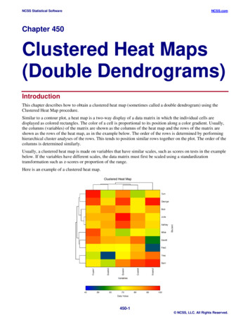
NCSS Statistical SoftwareNCSS.comChapter 450Clustered Heat Maps(Double Dendrograms)IntroductionThis chapter describes how to obtain a clustered heat map (sometimes called a double dendrogram) using theClustered Heat Map procedure.Similar to a contour plot, a heat map is a two-way display of a data matrix in which the individual cells aredisplayed as colored rectangles. The color of a cell is proportional to its position along a color gradient. Usually,the columns (variables) of the matrix are shown as the columns of the heat map and the rows of the matrix areshown as the rows of the heat map, as in the example below. The order of the rows is determined by performinghierarchical cluster analyses of the rows. This tends to position similar rows together on the plot. The order of thecolumns is determined similarly.Usually, a clustered heat map is made on variables that have similar scales, such as scores on tests in the examplebelow. If the variables have different scales, the data matrix must first be scaled using a standardizationtransformation such as z-scores or proportion of the range.Here is an example of a clustered heat map.450-1 NCSS, LLC. All Rights Reserved.

NCSS Statistical SoftwareNCSS.comClustered Heat Maps (Double Dendrograms)Hierarchical Clustering AlgorithmsThe cluster algorithms used for the rows and columns of the data matrix must be specified. NCSS allows you toselect from eight possible hierarchical algorithms. The clustering method selected for the columns need not be thesame as the method selected for the rows. Chapter 445 of the NCSS documentation gives an introduction tohierarchical clustering. Only highlights from that chapter are presented here.We will first give brief comments about each of the eight hierarchical clustering techniques.Group AverageAlso called the unweighted pair-group method, this is perhaps the most widely used of all the hierarchical clustertechniques. The distance between two groups is defined as the average distance between each of their members.Single LinkageAlso known as nearest neighbor clustering, this is one of the oldest and most famous of the hierarchicaltechniques. The distance between two groups is defined as the distance between their two closest members. Itoften yields clusters in which individuals are added sequentially to a single group.Complete LinkageAlso known as furthest neighbor or maximum method, this method defines the distance between two groups asthe distance between their two farthest-apart members. This method usually yields clusters that are well separatedand compact.Simple AverageAlso called the weighted pair-group method, this algorithm defines the distance between groups as the averagedistance between each of the members, weighted so that the two groups have an equal influence on the finalresult.CentroidAlso referred to as the unweighted pair-group centroid method, this method defines the distance between twogroups as the distance between their centroids (center of gravity or vector average). The method should only beused with Euclidean distances.Backward links may occur with this method. These are recognizable when the dendrogram no longer exhibits itssimple tree-like structure in which each fusion results in a new cluster that is at a higher distance level (movesfrom right to left). With backward links, fusions can take place that result in clusters at a lower distance level(move from left to right). The dendrogram is difficult to interpret in this case.MedianAlso called the weighted pair-group centroid method, this defines the distance between two groups as theweighted distance between their centroids, the weight being proportional to the number of individuals in eachgroup. Backward links (see discussion under Centroid) may occur with this method. The method should only beused with Euclidean distances.Ward’s Minimum VarianceWith this method, groups are formed so that the pooled within-group sum of squares is minimized. That is, ateach step, the two clusters are fused which result in the least increase in the pooled within-group sum of squares.450-2 NCSS, LLC. All Rights Reserved.

NCSS Statistical SoftwareNCSS.comClustered Heat Maps (Double Dendrograms)Flexible StrategyLance and Williams (1967) suggested that a continuum could be made between single and complete linkage. Theprogram lets you try various settings of these parameters which do not conform to the constraints suggested byLance and Williams.One interesting exercise is to vary these values, trying to find the set that maximizes the cophenetic correlationcoefficient.Goodness-of-FitGiven the large number of techniques, it is often difficult to decide which is best. One criterion that has becomepopular is to use the result that has largest cophenetic correlation coefficient. This is the correlation between theoriginal distances and those that result from the cluster configuration. Values above 0.75 are felt to be good. TheGroup Average method appears to produce high values of this statistic. This may be one reason that it is sopopular.A second measure of goodness of fit called delta is described in Mather (1976). These statistics measure degree ofdistortion rather than degree of resemblance (as with the cophenetic correlation). The two delta coefficients aregiven by N * 1/ A d jk - d jk j k A ( d*jk )1/ A j k A where A is either 0.5 or 1 and d ij* is the distance obtained from the cluster configuration. Values close to zero aredesirable.Mather (1976) suggests that the Group Average method is the safest to use as an exploratory method, although hegoes on to suggest that several methods should be tried and the one with the largest cophenetic correlation beselected for further investigation.DendrogramsThe agglomerative hierarchical clustering algorithms available in this program module build a cluster hierarchythat is commonly displayed as a tree diagram called a dendrogram. The algorithm begins by placing each objectin a separate cluster. Then, at each step, the two clusters that are most similar (according to a specific definition ofsimilarity) are joined into a single new cluster. Once fused, objects are never separated. The eight clusteringmethods that are available represent eight methods of defining the similarity between clusters.To help understand the dendrogram, consider the following example that has only two variables. Note that if wehad only two variables, we could perform the cluster analysis visually. The technique becomes useful once wehave three or more variables to consider.450-3 NCSS, LLC. All Rights Reserved.

NCSS Statistical SoftwareNCSS.comClustered Heat Maps (Double Dendrograms)Suppose we wish to cluster the bivariate data shown in the following scatter plot. In this case, the clustering maybe done visually. The data seem to exhibit three clusters and two singletons, 6 and 13.16.0Red vs Blue12.068.0358109117412134.0Blue2114 15 1617 18 190.020 21 220.05.010.015.020.0RedThe following dendrogram was produced from the above data using popular the Group Average 0The horizontal axis of the dendrogram represents the distance or dissimilarity between clusters. The vertical axisrepresents the objects and clusters. The dendrogram is fairly simple to interpret. Remember that our main interestis in similarity and clustering. Each joining (fusion) of two clusters is represented on the graph by the splitting ofa horizontal line into two horizontal lines. The horizontal position of the split, shown by the short vertical bar,gives the dissimilarity between the two clusters.Looking at this dendrogram, you can see the three clusters as three branches that occur at about the samehorizontal distance. The two outliers, 6 and 13, are added in rather arbitrarily at much higher distances. This is theinterpretation.In this example we can compare our interpretation with an actual plot of the data. Unfortunately, this usually willnot be possible because our data will consist of more than two variables.450-4 NCSS, LLC. All Rights Reserved.

NCSS Statistical SoftwareNCSS.comClustered Heat Maps (Double Dendrograms)Missing ValuesWhen an observation has missing values, appropriate adjustments are made so that the average dissimilarityacross all variables with non-missing data is computed. Hence, rows with missing values are not omitted unlessall variables have missing values. Note that the distances require that at least one variable have non-missingvalues for each pair of rows.Example 1 – Creating a Clustered Heat MapThis section presents an example of how to create a clustered heat map from a set of exam score data. The dataare found in the Exams database.SetupTo run this example, complete the following steps:1Open the Exams example dataset From the File menu of the NCSS Data window, select Open Example Data. 2Select Exams and click OK.Specify the Clustered Heat Maps (Double Dendrograms) procedure options Find and open the Clustered Heat Maps (Double Dendrograms) procedure using the menus or theProcedure Navigator. The settings for this example are listed below and are stored in the Example 1 settings template. To loadthis template, click Open Example Template in the Help Center or File menu.OptionValueVariables TabCluster Variable(s) . Exam1, Exam2, Exam3, Exam4, Exam5Row Label Variable . StudentVariable Scaling Method . NoneRow Scaling Method . NoneReports TabClustered Heat Map . CheckedCluster Reports . CheckedLinkage Reports. CheckedDistance Reports . Checked3Run the procedure Click the Run button to perform the calculations and generate the output.450-5 NCSS, LLC. All Rights Reserved.

NCSS Statistical SoftwareNCSS.comClustered Heat Maps (Double Dendrograms)Heat Map SectionClustered Heat Map This report displays the heat map for these data with the above settings. Note that the rows and columns havebeen sorted in the order specified by the clustering.Cluster Detail SectionCluster Detail Report when Clustering Variables Clustering Method Simple AverageDistance TypeEuclideanScale TypeNoneCluster12NoneVariables in this ClusterExam1, Exam3Exam4, Exam5Exam2Cluster Detail Report when Clustering Rows Clustering Method Simple AverageDistance TypeEuclideanScale TypeNoneCluster123Rows in ClusterTom, Bob, Julie, Ashley, GeorgeTina, SamMike, David, FredThis report displays the items contained in the row and variable clusters. Those items that cannot be classified arelisted in the ‘None’ cluster.450-6 NCSS, LLC. All Rights Reserved.