WIXLIB

SEC. 4.3COUNTING PERMUTATIONS161K’s and M’s and Powers of 2A useful trick for converting powers of 2 into decimal is to notice that 210 , or 1024,is very close to one thousand. Thus 230 is (210 )3 , or about 10003, that is, a billion.Then, 232 4 230 , or about four billion. In fact, computer scientists often acceptthe fiction that 210 is exactly 1000 and speak of 210 as “1K”; the K stands for “kilo.”We convert 215 , for example, into “32K,” because215 25 210 32 “1000”But 220 , which is exactly 1,048,576, we call “1M,” or “one million,” rather than“1000K” or “1024K.” For powers of 2 between 20 and 29, we factor out 220 . Thus,226 is 26 220 or 64 “million.” That is why 226 bytes is referred to as 64 millionbytes or 64 “megabytes.”Below is a table that gives the terms for various powers of 10 and their roughequivalents in powers of 2.PREFIXKiloMegaGigaTeraPetaLETTERKMGTPVALUE103 or 210106 or 220109 or 2301012 or 2401015 or 250This table suggests that for powers of 2 beyond 29 we factor out 230 , 240 , or 2raised to whatever multiple-of-10 power we can. The remaining powers of 2 namethe number of giga-, tera-, or peta- of whatever unit we are measuring. For example,243 bytes is 8 terabytes.O(n log n) time, are to within a constant factor as fast as can be.There are many other applications of the counting rule for permutations. Forexample, it figures heavily in more complex counting questions like combinationsand probabilities, as we shall see in later sections. Example 4.2. To develop some intuition, let us enumerate the permutations ofsmall numbers of objects. First, it should be clear that Π(1) 1. That is, if thereis only one object A, there is only one order: A.Now suppose there are two objects, A and B. We may select one of the twoobjects to be first and then the remaining object is second. Thus there are twoorders: AB and BA. Therefore, Π(2) 2 1 2.Next, let there be three objects: A, B, and C. We may select any of the threeto be first. Consider the case in which we select A to be first. Then the remainingtwo objects, B and C, can be arranged in either of the two orders for two objects tocomplete the permutation. We thus see that there are two orders that begin withA, namely ABC and ACB.Similarly, if we start with B, there are two ways to complete the order, corre-

162COMBINATORICS AND PROBABILITYsponding to the two ways in which we may order the remaining objects A and C.We thus have orders BAC and BCA. Finally, if we start with C first, we can orderthe remaining objects A and B in the two possible ways, giving us orders CAB andCBA. These six orders,ABC, ACB, BAC, BCA, CAB, CBAare all the possible orders of three elements. That is, Π(3) 3 2 1 6.Next, consider how many permutations there are for 4 objects: A, B, C, andD. If we pick A first, we may follow A by the objects B, C, and D in any of their6 orders. Similarly, if we pick B first, we can order the remaining A, C, and D inany of their 6 ways. The general pattern should now be clear. We can pick anyof the four elements first, and for each such selection, we can order the remainingthree elements in any of the Π(3) 6 possible ways. It is important to note thatthe number of permutations of the three objects does not depend on which threeelements they are. We conclude that the number of permutations of 4 objects is 4times the number of permutations of 3 objects. More generally,Π(n 1) (n 1)Π(n) for any n 1(4.1)That is, to count the permutations of n 1 objects we may pick any of the n 1objects to be first. We are then left with n remaining objects, and these can bepermuted in Π(n) ways, as suggested in Fig. 4.4. For our example where n 1 4,we have Π(4) 4 Π(3) 4 6 24.First objectObject 1Object 2n remaining objectsΠ(n)ordersΠ(n)orders.Object n 1Π(n)ordersFig. 4.4. The permutations of n 1 objects.

SEC. 4.3COUNTING PERMUTATIONS163The Formula for PermutationsEquation (4.1) is the inductive step in the definition of the factorial function introduced in Section 2.5. Thus it should not be a surprise that Π(n) equals n!. We canprove this equivalence by a simple induction.STATEMENTS(n): Π(n) n! for all n 1.For n 1, S(1) says that there is 1 permutation of 1 object. We observedthis simple point in Example 4.2.BASIS.INDUCTION. Suppose Π(n) n!. Then S(n 1), which we must prove, says thatΠ(n 1) (n 1)!. We start with Equation (4.1), which says thatΠ(n 1) (n 1) Π(n)By the inductive hypothesis, Π(n) n!. Thus, Π(n 1) (n 1)n!. Sincen! n (n 1) · · · 1it must be that (n 1) n! (n 1) n (n 1) · · · 1. But the latter productis (n 1)!, which proves S(n 1). Example 4.3. As a result of the formula Π(n) n!, we conclude that thenumber of permutations of 4 objects is 4! 4 3 2 1 24, as we saw above.As another example, the number of permutations of 7 objects is 7! 5040. How Long Does it Take to Sort?Generalpurpose sortingalgorithmOne of the interesting uses of the formula for counting permutations is in a proofthat sorting algorithms must take at least time proportional to n log n to sort nelements, unless they make use of some special properties of the elements. Forexample, as we note in the box on special-case sorting algorithms, we can do betterthan proportional to n log n if we write a sorting algorithm that works only for smallintegers.However, if a sorting algorithm works on any kind of data, as long as it canbe compared by some “less than” notion, then the only way the algorithm candecide on the proper order is to consider the outcome of a test for whether oneof two elements is less than the other. A sorting algorithm is called a generalpurpose sorting algorithm if its only operation upon the elements to be sorted is acomparison between two of them to determine their relative order. For instance,selection sort and merge sort of Chapter 2 each make their decisions that way. Eventhough we wrote them for integer data, we could have written them more generallyby replacing comparisons likeif (A[j] A[small])on line (4) of Fig. 2.2 by a test that calls a Boolean-valued function such asif (lessThan(A[j], A[small]))

164COMBINATORICS AND PROBABILITYSuppose we are given n distinct elements to sort. The answer — that is, thecorrect sorted order — can be any of the n! permutations of these elements. If ouralgorithm for sorting arbitrary types of elements is to work correctly, it must beable to distinguish all n! different possible answers.Consider the first comparison of elements that the algorithm makes, saylessThan(X,Y)For each of the n! possible sorted orders, either X is less than Y or it is not. Thus,the n! possible orders are divided into two groups, those for which the answer tothe first test is “yes” and those for which it is “no.”One of these groups must have at least n!/2 members. For if both groups havefewer than n!/2 members, then the total number of orders is less than n!/2 n!/2,or less than n! orders. But this upper limit on orders contradicts the fact that westarted with exactly n! orders.Now consider the second test, on the assumption that the outcome of thecomparison between X and Y was such that the larger of the two groups of possibleorders remains (take either outcome if the groups are the same size). That is, atleast n!/2 orders remain, among which the algorithm must distinguish. The secondcomparison likewise has two possible outcomes, and at least half the remainingorders will be consistent with one of these outcomes. Thus, we can find a group ofat least n!/4 orders consistent with the first two tests.We can repeat this argument until the algorithm has determined the correctsorted order. At each step, by focusing on the outcome with the larger populationof consistent possible orders, we are left with at least half as many possible orders asat the previous step. Thus, we can find a sequence of tests and outcomes such thatafter the ith test, there are at least n!/2i orders consistent with all these outcomes.Since we cannot finish sorting until every sequence of tests and outcomes isconsistent with at most one sorted order, the number of tests t made before wefinish must satisfy the equationn!/2t 1(4.2)If we take logarithms base 2 of both sides of Equation (4.2) we have log2 n! t 0,ort log2 (n!)We shall see that log2 (n!) is about n log2 n. But first, let us consider an example ofthe process of splitting the possible orders. Example 4.3. Let us consider how the selection sort algorithm of Fig. 2.2makes its decisions when given three elements (a, b, c) to sort. The first comparisonis between a and b, as suggested at the top of Fig. 4.5, where we show in the boxthat all 6 possible orders are consistent before we make any tests. After the test,the orders abc, acb, and cab are consistent with the “yes” outcome (i.e., a b),while the orders bac, bca, and cba are consistent with the opposite outcome, whereb a. We again show in a box the consistent orders in each case.In the algorithm of Fig. 2.2, the index of the smaller becomes the value small.Thus, we next compare c with the smaller of a and b. Note that which test is madenext depends on the outcome of previous tests.

SEC. 4.3COUNTING PERMUTATIONS165After making the second decision, the smallest of the three is moved into thefirst position of the array, and a third comparison is made to determine which ofthe remaining elements is the larger. That comparison is the last comparison madeby the algorithm when three elements are to be sorted. As we see at the bottomof Fig. 4.5, sometimes that decision is determined. For example, if we have alreadyfound a b and c a, then c is the smallest and the last comparison of a and bmust find a smaller.abc, acb, bac, bca, cab, cbaa b?YNabc, acb, caba c?Yabc, acbYb c?abcNacbYcabbac, bca, cbab c?NYcabbac, bcaa b?NYbaca c?NbcaNcbaYa b?NcbaFig. 4.5. Decision tree for selection sorting of 3 elements.In this example, all paths involve 3 decisions, and at the end there is at mostone consistent order, which is the correct sorted order. The two paths with noconsistent order never occur. Equation (4.2) tells us that the number of tests tmust be at least log2 3!, which is log2 6. Since 6 is between 22 and 23 , we know thatlog2 6 will be between 2 and 3. Thus, at least some sequences of outcomes in anyalgorithm that sorts three elements must make 3 tests. Since selection sort makesonly 3 tests for 3 elements, it is at least as good as any other sorting algorithm for 3elements in the worst case. Of course, as the number of elements becomes large, weknow that selection sort is not as good as can be done, since it is an O(n2 ) sortingalgorithm and there are better algorithms such as merge sort. We must now estimate how large log2 n! is. Since n! is the product of all theintegers from 1 to n, it is surely larger than the product of only the n2 1 integersfrom n/2 through n. This product is in turn at least as large as n/2 multiplied byitself n/2 times, or (n/2)n/2 . Thus, log2 n! is at least log2 (n/2)n/2 . But the latteris n2 (log2 n log2 2), which isn(log2 n 1)2For large n, this formula is approximately (n log2 n)/2.A more careful analysis will tell us that the factor of 1/2 does not have to bethere. That is, log2 n! is very close to n log2 n rather than to half that expression.

166COMBINATORICS AND PROBABILITYA Linear-Time Special-Purpose Sorting AlgorithmIf we restrict the inputs on which a sorting algorithm will work, it can in one stepdivide the possible orders into more than 2 parts and thus work in less than timeproportional to n log n. Here is a simple example that works if the input is n distinctintegers, each chosen in the range 0 to 2n 1.(1)(2)(3)(4)(5)(6)(7)for (i 0; i 2*n; i )count[i] 0;for (i 0; i n; i )count[a[i]] ;for (i 0; i 2*n; i )if (count[i] 0)printf("%d\n", i);We assume the input is in an array a of length n. In lines (1) and (2) weinitialize an array count of length 2n to 0. Then in lines (3) and (4) we add 1to the count for x if x is the value of a[i], the ith input element. Finally, inthe last three lines we print each of the integers i such that count[i] is positive.Thus we print those elements appearing one or more times in the input and, on theassumption the inputs are distinct, it prints all the input elements, sorted smallestfirst.We can analyze the running time of this algorithm easily. Lines (1) and (2)are a loop that iterates 2n times and has a body taking O(1) time. Thus, it takesO(n) time. The same applies to the loop of lines (3) and (4), but it iterates n timesrather than 2n times; it too takes O(n) time. Finally, the body of the loop of lines(5) through (7) takes O(1) time and it is iterated 2n times. Thus, all three loopstake O(n) time, and the entire sorting algorithm likewise takes O(n) time. Notethat if given an input for which the algorithm is not tailored, such as integers in arange larger than 0 through 2n 1, the program above fails to sort correctly.We have shown only that any general-purpose sorting algorithm must havesome input for which it makes about n log2 n comparisons or more. Thus anygeneral-purpose sorting algorithm must take at least time proportional to n log nin the worst case. In fact, it can be shown that the same applies to the “average”input. That is, the average over all inputs of the time taken by a general-purposesorting algorithm must be at least proportional to n log n. Thus, merge sort is aboutas good as we can do, since it has this big-oh running time for all inputs.EXERCISES4.3.1: Suppose we have selected 9 players for a baseball team.a)b)How many possible batting orders are there?If the pitcher has to bat last, how many possible batting orders are there?4.3.2: How many comparisons does the selection sort algorithm of Fig. 2.2 makeif there are 4 elements? Is this number the best possible? Show the top 3 levels ofthe decision tree in the style of Fig. 4.5.

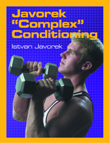
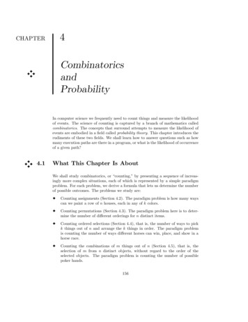
SEC. 4.4ORDERED SELECTIONS1674.3.3: How many comparisons does the merge sort algorithm of Section 2.8 makeif there are 4 elements? Is this number the best possible? Show the top 3 levels ofthe decision tree in the style of Fig. 4.5.4.3.4*: Are there more assignments of n values to n items or permutations of n 1items? Note: The answer may not be the same for all n.4.3.5*: Are there more assignments of n/2 values to n items than there are permutations of n items?4.3.6**: Show how to sort n integers in the range 0 to n2 1 in O(n) time. 4.4Ordered SelectionsSometimes we wish to select only some of the items in a set and give them an order.Let us generalize the function Π(n) that counted permutations in the previoussection to a two-argument function Π(n, m), which we define to be the number ofways we can select m items from n in such a way that order matters for the selecteditems, but there is no order for the unselected items. Thus, Π(n) Π(n, n). Example 4.5. A horse race awards prizes to the first three finishers; the firsthorse is said to “win,” the second to “place,” and the third to “show.” Supposethere are 10 horses in a race. How many different awards for win, place, and showare there?Clearly, any of the 10 horses can be the winner. Given which horse is thewinner, any of the 9 remaining horses can place. Thus, there are 10 9 90choices for horses in first and second positions. For any of these 90 selections ofwin and place, there are 8 remaining horses. Any of these can finish third. Thus,there are 90 8 720 selections of win, place, and show. Figure 4.6 suggests allthese possible selections, concentrating on the case where 3 is selected first and 1 isselected second. The General Rule for Selections Without ReplacementLet us now deduce the formula for Π(n, m). Following Example 4.5, we know thatthere are n choices for the first selection. Whatever selection is first made, therewill be n 1 remaining items to choose from. Thus, the second choice can be madein n 1 different ways, and the first two choices occur in n(n 1) ways. Similarly,for the third choice we are left with n 2 unselected items, so the third choicecan be made in n 2 different ways. Hence the first three choices can occur inn(n 1)(n 2) distinct ways.We proceed in this way until m choices have been made. Each choice is madefrom one fewer item than the choice before. The conclusion is that we may selectm items from n without replacement but with order significant inΠ(n, m) n(n 1)(n 2) · · · (n m 1)(4.3)different ways. That is, expression (4.3) is the product of the m integers startingand n and counting down.Another way to write (4.3) is as n!/(n m)!. That is,

168COMBINATORICS AND PROBABILITY1.2.All but 1All but 224513.2.4.All but 3, 4.All but 3, 10.1010.10All but 2, 3All but 10Fig. 4.6. Ordered selection of three things out of 10.n(n 1) · · · (n m 1)(n m)(n m 1) · · · (1)n! (n m)!(n m)(n m 1) · · · (1)The denominator is the product of the integers from 1 to n m. The numeratoris the product of the integers from 1 to n. Since the last n m factors in thenumerator and denominator above are the same, (n m)(n m 1) · · · (1), theycancel and the result is thatn! n(n 1) · · · (n m 1)(n m)!This formula is the same as that in (4.3), which shows that Π(n, m) n!/(n m)!. Example 4.6. Consider the case from Example 4.5, where n 10 and m 3. We observed that Π(10, 3) 10 9 8 720. The formula (4.3) says thatΠ(10, 3) 10!/7!, or

SEC. 4.4ORDERED SELECTIONS169Selections With and Without ReplacementSelection withreplacementSelectionwithoutreplacementThe problem considered in Example 4.5 differs only slightly from the assignmentproblem considered in Section 4.2. In terms of houses and colors, we could almostsee the selection of the first three finishing horses as an assignment of one of tenhorses (the “colors”) to each of three finishing positions (the “houses”). The onlydifference is that, while we are free to paint several houses the same color, it makesno sense to say that one horse finished both first and third, for example. Thus, whilethe number of ways to color three houses in any of ten colors is 103 or 10 10 10,the number of ways to select the first three finishers out of 10 is 10 9 8.We sometimes refer to the kind of selection we did in Section 4.2 as selectionwith replacement. That is, when we select a color, say red, for a house, we “replace”red into the pool of possible colors. We are then free to select red again for one ormore additional houses.On the other hand, the sort of selection we discussed in Example 4.5 is calledselection without replacement. Here, if the horse Sea Biscuit is selected to be thewinner, then Sea Biscuit is not replaced in the pool of horses that can place orshow. Similarly, if Secretariat is selected for second place, he is not eligible to bethe third-place horse also.10 9 8 7 6 5 4 3 2 17 6 5 4 3 2 1The factors from 1 through 7 appear in both numerator and denominator and thuscancel. The result is the product of the integers from 8 through 10, or 10 9 8,as we saw in Example 4.5. EXERCISES4.4.1: How many ways are there to form a sequence of m letters out of the 26letters, if no letter is allowed to appear more than once, for (a) m 3 (b) m 5.4.4.2: In a class of 200 studen

rudiments of these two fields. We shall learn how to answer questions such as how many execution paths are there in a program, or what is the likelihood of occurrence of a given path? 4.1 What This Chapter Is About We shall study combinato