Transcription
Mathematical Methods of Operations Research (2022) 77-xORIGINAL ARTICLEGenerative deep learning for decision making in gasnetworksLovis Anderson2· Mark Turner1,2· Thorsten Koch1,2Received: 28 January 2021 / Revised: 3 February 2022 / Accepted: 23 February 2022 /Published online: 19 April 2022 The Author(s) 2022AbstractA decision support system relies on frequent re-solving of similar problem instances.While the general structure remains the same in corresponding applications, the inputparameters are updated on a regular basis. We propose a generative neural networkdesign for learning integer decision variables of mixed-integer linear programming(MILP) formulations of these problems. We utilise a deep neural network discriminatorand a MILP solver as our oracle to train our generative neural network. In this article,we present the results of our design applied to the transient gas optimisation problem.The trained generative neural network produces a feasible solution in 2.5s, and whenused as a warm start solution, decreases global optimal solution time by 60.5%.Keywords Mixed-integer programming · Deep learning · Primal heuristic · Gasnetworks · Generative modellingThe work for this article has been conducted in the Research Campus MODAL funded by the GermanFederal Ministry of Education and Research (BMBF) (fund numbers 05M14ZAM, 05M20ZBM), and wassupported by the German Federal Ministry of Economic Affairs and Energy (BMWi) through the projectUNSEEN (fund no 03EI1004D): Bewertung der Unsicherheit in linear optimiertenEnergiesystem-Modellen unter Zuhilfenahme Neuronaler Netze.BMark Turnerturner@zib.deLovis Andersonanderson@zib.deThorsten Kochkoch@zib.de1Chair of Software and Algorithms for Discrete Optimization, Institute of Mathematics,Technische Universität Berlin, Straße des 17. Juni 135, 10623 Berlin, Germany2Applied Algorithmic Intelligence Methods Department, Zuse Institute Berlin, Takustr. 7, 14195Berlin, Germany123
504L. Anderson et al.1 IntroductionMixed-Integer Linear Programming (MILP) is concerned with the modelling andsolving of problems from discrete optimisation. These problems can represent realworld scenarios, where discrete decisions can be appropriately captured and modelledby integer variables. In real-world scenarios a MILP model is rarely solved onlyonce. More frequently, the same model is used with varying data to describe differentinstances of the same problem, which are solved on a regular basis. This holds truein particular for decision support systems, which can utilise MILP to provide realtime optimal decisions on a continual basis, see (Beliën et al. 2009) and (Ruiz et al.2004) for examples in nurse scheduling and vehicle routing. The MILPs that thesedecision support systems solve have identical structure due to both their underlyingapplication and cyclical nature, and thus often have similar optimal solutions. Ouraim is to exploit this repetitive structure, and create generative neural networks thatgenerate binary decision encodings for subsets of important variables. These encodings can be used in a primal heuristic by solving the induced subproblem followingvariable fixations. Additionally, the result of the primal heuristic can be used in awarm start context to help improve solver performance in achieving global optimality.We demonstrate the performance of our neural network (NN) design on the transientgas optimisation problem (Ríos-Mercado and Borraz-Sánchez 2015), specifically onreal-world instances embedded in day ahead decision support systems.The design of our framework is inspired by the recent development of GenerativeAdversarial Networks (GANs) (Goodfellow 2016). Our design consists of two NNs,a generator and a discriminator. The generator is responsible for generating binarydecision values, while the discriminator is tasked with predicting the optimal objectivefunction value of the reduced MILP that arises after fixing these binary variables totheir generated values. Our NN design and its application to transient gas networkMILP formulations is an attempt to integrate Machine Learning (ML) into the MILPsolving process. This integration has recently received an increased focus (Tang et al.2019; Bertsimas and Stellato 2019; Gasse et al. 2019), which has been encouragedby the success of ML integration into other aspects of combinatorial optimisation, see(Bengio et al. 2018) for a thorough overview.The paper is structured as follows: Sect. 2 contains an overview of the literaturewith comparisons to our work. In Sect. 3, we introduce our main contribution, a newgenerative NN design for learning binary variables of parametric MILPs. Afterward,we outline a novel data generation approach for generating synthetic gas transportinstances in Sect. 4. Section 5 outlines the exact training scheme for our new NN andhow our framework can be used to warm start MILPs. Finally, in Sect. 6, we showand discuss the results of our NN design on real-world gas transport instances. Thisrepresents a major contribution, as the trained NN generates a primal solution in 2.5sand via warm start reduces solution time to achieve global optimality by 60.5%.123
Generative deep learning for decision making in gas networks5052 Background and related workAs mentioned in the introduction, the intersection of MILP and ML is currently an areaof active and growing research. For a thorough overview of deep learning (DL), therelevant subset of ML used throughout this article, we refer readers to Goodfellow et al.(2016), and for MILP to Achterberg (2007). We will highlight previous research fromthis intersection that we believe is either tangential, or may have shared applicationsto that presented in this paper. Additionally, we will briefly detail the state-of-the-artin transient gas transport, and highlight why our design is of practical importance. Itshould be noted as well that there are recent research activities aiming at the reversedirection, with MILP applied to ML instead of the orientation we consider, see (Wongand Kolter 2017) for an interesting example.Firstly, we summarise applications of ML to adjacent areas of the MILP solvingprocess. Gasse et al. (2019) creates a method for encoding MILP structure in a bipartite graph representing variable-constraint relationships. This structure is the input toa Graph Convolutional Neural Network (GCNN), which imitates strong branchingdecisions. The strength of their results stem from intelligent network design and thegeneralisation of their GCNN to problems of a larger size, albeit with some generalisation loss. Zarpellon et al. (2020) take a different approach, and use a NN designthat incorporates the branch-and-bound tree state directly. In doing so, they show thatinformation contained in the global branch-and-bound tree state is an important factorin variable selection. Furthermore, their publication is one of the few to present resultson heterogeneous instances. Etheve et al. (2020) show a successful implementationof reinforcement learning for variable selection. Tang et al. (2019) show preliminary results of how reinforcement learning can be used in cutting plane selection.By restricting themselves exclusively to Gomory cuts, they are able to produce anagent capable of selecting better cuts than default solver settings for specific classesof problems.There exists a continuous trade-off between model fidelity and complexity in thefield of transient gas optimisation, and there is no standard model for transient gastransport problems. Moritz (2007) presents a piecewise linear MILP approach to thetransient gas transport problem, (Burlacu et al. 2019) a nonlinear approach with anovel discretisation scheme, and (Hennings et al. 2020) and (Hoppmann et al. 2019)a linearised approach. For the purpose of our experiments, we use the model of Hennings et al. (2020), which uses linearised equations and focuses on gas subnetworkswith many controllable elements. The current research of ML in gas transport is still inthe early stages. Pourfard et al. (2019) use a dual NN design to perform online calculations of a compressors operating point to avoid re-solving the underlying model. Theapproach constrains itself to continuous variables and experimental results are presented for a gunbarrel gas network. MohamadiBaghmolaei et al. (2014) present a NNcombined with a genetic algorithm for learning the relationship between compressorspeeds and the fuel consumption rate in the absence of complete data. More often, MLhas been used in fields closely related to gas transport, as in Hanachi et al. (2018), withML used to track the degradation of compressor performance, and in Petkovic et al.(2019) to forecast demand values at the boundaries of the gas network. For a more123
506L. Anderson et al.complete overview of the transient gas literature, we refer readers to Ríos-Mercadoand Borraz-Sánchez (2015).Our framework, which predicts the optimal objective value of an induced subMILP, can be considered similar to Baltean-Lugojan et al. (2019) in what it predictsand similar to Ferber et al. (2019), in how it works. In the first paper (Baltean-Lugojanet al. 2019), a NN is used to predict the associated objective value improvements oncuts. This is a smaller scope than our prediction, but is still heavily concerned with theMILP formulation. In the second paper (Ferber et al. 2019), a technique is developedthat performs backward passes directly through a MILP. It does this by solving MILPsexclusively with cutting planes, and then receiving gradient information from the KKTconditions of the final linear program. This application of a NN, which produces inputto the MILP, is very similar to our design. The differences arise in that we rely on a NNdiscriminator to appropriately distribute the loss instead of solving a MILP directly,and that we generate variable values instead of parameter values with our generator.While our framework is heavily inspired from GANs (Goodfellow 2016), it is alsosimilar to actor-critic algorithms, see (Pfau and Vinyals 2016). These algorithms haveshown success for variable generation in MILP, and are notably different in that theysample from a generated distribution for downstream decisions instead of alwaystaking the decision with highest probability. Recently, (Chen et al. 2020) generated aseries of coordinates for a set of UAVs using an actor-critic based algorithm, wherethese coordinates were continuous variables in a Mixed-Integer Non-Linear Program(MINLP) formulation. The independence of separable subproblems and the easilyrealisable value function within their formulation resulted in a natural Markov DecisionProcess interpretation. For a better comparison on the similarities between actor-criticalgorithms and GANs, we refer readers to Pfau and Vinyals (2016).Finally, we summarise existing research that also deals with the generation ofdecision variable values for Mixed-Integer Programs. Bertsimas and Stellato (2018,2019) attempt to learn optimal solutions of parametric MILPs and Mixed-IntegerQuadratic Programs (MIQPs), which involves both outputting all integer decisionvariable values and the active set of constraints. They mainly use optimal classificationtrees in Bertsimas and Stellato (2018) and NNs in Bertsimas and Stellato (2019). Theiraim is tailored towards smaller problems classes, where speed is an absolute priorityand parameter value changes are limited. Masti and Bemporad (2019) learn binarywarm start decisions for MIQPs. They use NNs with a loss function that combinesbinary cross entropy and a penalty for infeasibility. Their goal of obtaining a primalheuristic is similar to ours, and while their design is much simpler, it has been shown towork effectively on very small problems. Our improvement over this design is our nonreliance on labelled optimal solutions, which are needed for binary cross entropy. Dinget al. (2019) present a GCNN design which is an extension of Gasse et al. (2019), anduse it to generate binary decision variable values. Their contributions are a tripartitegraph encoding of MILP instances, and the inclusion of their aggregated generatedvalues as branching decisions in the branch-and-bound tree, both in an exact approachand in an approximate approach with local branching (Fischetti and Lodi 2003). Veryrecently, (Nair et al. 2020) combined the branching approach of Gasse et al. (2019) witha novel neural diving approach, in which integer variable values are generated. Theyuse a GCNN for generating both branching decisions and integer variables values.123
Generative deep learning for decision making in gas networks507Different to our generator-discriminator based approach, they generate values directlyfrom a learned distribution, which is based on an energy function that incorporatesresulting objective values.3 The solution frameworkWe begin by formally defining both a MILP and a NN. Our definition of a MILP is anextension of more traditional formulations, see (Achterberg 2007), but still encapsulates general instances.Definition 1 Let π R p be a vector of problem-defining parameters, where p Z 0 .We use π as a subscript to indicate that a variable is parameterised by π . We call Pπa MILP parameterised by π . min s.t.Pπ : c1T x1 c2T x2 c3T z 1 c4T z 2 x1 x 2 Aπ bπ z1 z2ck Rn k , k {1, 2, 3, 4}, Aπ Rm n , bπ Rmx1 Rn 1 , x2 Rn 2 , z 1 {0, 1}n 3 , z 2 {0, 1}n 4 , n k Z 0Furthermore let R p be a set of valid problem-defining parameters. We then call{Pπ π } a problem class for . Lastly, we denote the optimal objective functionvalue of Pπ by f (Pπ ).Note that the explicit parameter space is usually unknown, but we assume in thefollowing to have access to a random variable that samples from . In addition,note that ci and n i are not parameterised by π , and as such the objective functionand variable dimensions do not change between scenarios. In Definition 3 we definean oracle NN Gθ1 , which predicts a subset of the binary variables of Pπ , namely z 1 .Additionally, the continuous variables x2 are separated in order to differentiate theslack variables in our example, which we will introduce in Sect. 4.We now provide a simple definition for feed forward NNs. For a larger variety ofdefinitions, see (Goodfellow et al. 2016).Definition 2 Let Nθ be defined by: R ak 1 ; a1 Nθ (a1 ) ak 1Nθ : R a1 h i : R ai R ai i {2, ., k 1}ai 1 : h i 1 (Wi ai bi ) i {1, ., k}(1)Wi R ai 1 ai , bi R ai 1 i {1, ., k}123
508L. Anderson et al.Fig. 1 The general design of N{θ1 ,θ2 }We then call Nθ a k-layer feed forward NN. Here, θ is the vector of all weights Wi andbiases bi of the NN. The functions h i are non-linear element-wise functions, calledactivation functions. Additionally, ai , bi , and Wi are tensors for all i {1, . . . , k}.Definition 3 For a problem class {Pπ π }, let the generator Gθ1 be a NNpredicting z 1 , and the discriminator Dθ2 be a NN predicting f (Pπ ) for π , i.e.Gθ1 : R p (0, 1)n 3Dθ2 : (0, 1)n 3 R p R(2)Furthermore, a forward pass of both Gθ1 and Dθ2 is defined as follows:zˆ1 : Gθ1 (π )(3)fˆ(Pπzˆ1 ) : Dθ2 (zˆ1 , π )(4)The hat notation is used to denote quantities that were approximated by a NN. We usesuperscript notation to create the following instances:Pπzˆ1 : Pπ s.t. z 1 [zˆ1 ](5)The additional notation of the square brackets around zˆ1 , refers to the rounding ofvalues from the range (0, 1) to {0, 1}, which is required as the variable values must bebinary.The goal of this framework is to generate good initial solution values zˆ1 , whichlead to an induced sub-MILP, Pπzˆ1 , whose optimal solution is a good feasible solutionto the original problem Pπ . Further, the idea is to use this feasible solution as a firstincumbent for warm starting the solution process of Pπ . To ensure feasibility for allchoices of z 1 , we divide the continuous variables into two sets, x1 and x2 , as seen inDefinition 1. The variables x2 are potential slack variables that ensure all generateddecisions result in feasible Pπzˆ1 instances, and are penalised in the objective. We nowdescribe the design of Gθ1 and Dθ2 .123
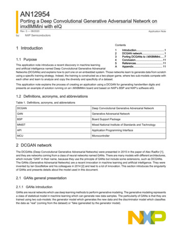
Generative deep learning for decision making in gas networks509Fig. 2 Method of merging two 1-D input streams3.1 Generator and discriminator designGθ1 and Dθ2 are NNs whose structure is inspired by Goodfellow (2016), as well as bothinception blocks and residual NNs, which have greatly increased large-scale modelperformance (Szegedy et al. 2017). We use the block design Resnet-v2 from Szegedyet al. (2017), see Fig. 3, albeit with a modification that primarily uses 1-D convolutions,with that dimension being time. Additionally, we separate initial input streams bytheir characteristics, and when joining two streams use 2-D convolutions. These 2-Dconvolutions reduce the data back to 1-D, see Fig. 2 for an visualisation of this process.The final layer of Gθ1 contains a softmax activation function with temperature. As thesoftmax temperature parameter increases, this activation function’s output approachesa one-hot vector encoding. The final layer of Dθ2 contains a softplus activation function.All other intermediate layers use the ReLU activation function. We refer readers toGoodfellow et al. (2016) for a thorough overview of deep learning, and to Fig. 14 inAppendix 1 for our complete design.For a vector x (x1 , · · · , xn ), the softmax function with temperature T R,σ1 , the ReLU function, σ2 , and the softplus function with parameter β R, σ3 , aredefined as:σ1 (xi , T ) : exp(T xi )nj 1 exp(T x j )σ2 (xi ) : max(0, xi )1σ3 (xi , β) : log(1 exp(βxi ))β(6)(7)(8)We compose Gθ1 and Dθ2 to make N{θ1 ,θ2 } . The definition of this composition isgiven in (9), and a visualisation in Fig. 1.N{θ1 ,θ2 } (π ) : Dθ2 (Gθ1 (π ), π )(9)3.2 InterpretationsIn a similar manner to GANs and actor-critic algorithms, see (Pfau and Vinyals 2016),the design of N{θ1 ,θ2 } has a bi-level optimisation interpretation, see (Dempe 2002) foran overview of bi-level optimisation. Here we list the explicit objectives of both Gθ1and Dθ2 , and how their loss functions represent these objectives.123
510L. Anderson et al.Fig. 3 1-D Resnet-v2 Block DesignThe objective of Dθ2 is to predict f (Pπzˆ1 ), the optimal induced objective value ofIts loss function is thus:Pπzˆ1 .Gθ1 (π )L(θ2 , π ) : Dθ2 (Gθ1 (π ), π ) f (Pπ)(10)The objective of Gθ1 is to minimise the induced prediction of Dθ2 . Its loss functionis thus:L (θ1 , π ) : Dθ2 (Gθ1 (π ), π )123(11)
Generative deep learning for decision making in gas networks511The corresponding bi-level optimisation problem can then be viewed as:min Eπ [Dθ2 (Gθ1 (π ), π )]θ1Gθ1 (π )s.t. min Eπ [ Dθ2 (Gθ1 (π ), π ) f (Pπθ2(12)) ]3.3 Training methodFor effective training of Gθ1 , a capable Dθ2 is needed. We therefore pre-train Dθ2 . Thefollowing loss function, which replaces Gθ1 (π ) with synthetic z 1 values in (10), isused for this pre-training:L (θ2 , π ) : Dθ2 (z 1 , π ) f (Pπz 1 )(13)However, performing this initial training requires generating instances of Pπz 1 , and istherefore done in a supervised manner offline manner on synthetic data.After the initial training of Dθ2 , we train Gθ1 as a part of N{θ1 ,θ2 } , using samplesπ , the loss function (11), and fixed θ2 . The issue of Gθ1 outputting continuousvalues for zˆ1 is overcome by the choice of the final activation function of Gθ1 . Thesoftmax with temperature (6) ensures that adequate gradient information still exists toupdate θ1 , and that the results are near binary. When using these results to explicitlysolve Pπzˆ1 , we round our result to a one-hot vector encoding along the appropriatedimension.After the completion of both initial trainings, we alternatingly train both NNs usingupdated loss functions in the following way:– Dθ2 training:– As in the initial training, using loss function (13).– In an online fashion, using predictions from Gθ1 and loss function (10).– Gθ1 training:– As explained above with loss function (11).Our design allows the loss to be back-propagated through Dθ2 and distributed to theindividual nodes of the final layer of Gθ1 that correspond to z 1 . This is largely differentto other methods, many of which rely on using loss against optimal solutions of Pπ ,see (Masti and Bemporad 2019; Ding et al. 2019). Our advantage over these is that thecontribution to fˆ(Pπzˆ1 ) of each predicted decision zˆ1 can be calculated. Additionally,we believe that it makes our generated suboptimal solutions more likely to be nearoptimal. We believe this because the NN is trained to minimise a predicted objectiverather than copy previously observed optimal solutions.123
512L. Anderson et al.4 The gas transport model and data generationTo evaluate the performance of our approach, we test our framework on the transient gas optimisation problem, see (Ríos-Mercado and Borraz-Sánchez 2015) for anoverview of the problem and associated literature. This problem is difficult to solve as itcombines a transient flow problem with complex combinatorics representing switchingdecisions. The natural modelling of transient gas networks as time-expanded networkslends itself well to our framework, however, due to the static underlying gas networkand repeated constraints at each time step. In this section we summarise importantaspects of our MILP formulation, and outline our methods for generating artificial gastransport data.4.1 The gas transport modelWe use the description of transient gas networks by Hennings et al. (2020). Thismodel contains operation modes, which are binary decisions corresponding to thez 1 of Definition 1. Exactly one operation mode is selected each time step, and thisdecision decides on the discrete states of all controllable elements in the gas networkfor that time step. We note that we deviate slightly from the model by Hennings et al.(2020), and do not allow the inflow over a set of entry-exits to be freely distributedaccording to which group they belong. This is an important distinction as each singleexit-entry in our model has a complete forecast.The model by Hennings et al. (2020) contains slack variables that change the pressure and flow demand scenarios at entry-exits. These slack variables are representedby x2 in Definition 1, and because of their existence we have yet to find an infeasibleinstance Pπz 1 for any choice of z 1 . We believe that infeasible scenarios can be inducedwith sufficiently small time steps, but this is not the case in our experiments. The slackvariables x2 are penalised in the objective.4.2 Data generationIn this subsection we outline our methods for generating synthetic transient gasinstances for training purposes, i.e. generating π and artificial z 1 values. Section4.2.1 introduces a novel method for generating balanced demand scenarios, followedby Sect. 4.2.2 that outlines how to generate operation mode sequences. Afterward,Sect. 4.2.3 presents an algorithm, which generates initial states of a gas network.These methods are motivated by the lack of available gas network data, see (Yueksel Erguen et al. 2020; Kunz et al. 2017), and the need for large amounts of data totrain our NN.4.2.1 Boundary forecast generationLet dv,t R, be the flow demand of entry-exit v V b at a time t T , where V b arethe set of entry-exit nodes and T is our discrete time horizon. Note that in Henningset al. (2020), these variables are written with hat notation, but we have omitted them123
Generative deep learning for decision making in gas networks513to avoid confusion with predicted values. We generate a balanced demand scenario,where the demands are bounded by the largest historically observed values, and thedemand between time steps has a maximal change. Additionally, two entry or exitsfrom the same fence group, g G, see (Hennings et al. 2020), have maximal demanddifferences within the same time step. Let I denote the set of real-world instances,where the superscript i I indicates that the value is an observed value in real-worldinstance i, and the superscript ‘sample’ indicates the value is sampled. A completesamplevalues for all v V b and t T that satisfy theflow forecast consists of dv,tfollowing constraints: sampledv,t 0 t T(14)v V bMq i dv,t 2121 Mq , Mq2020sampledv,tmaxv V b ,t T ,i Isample dv,tsample dv,t 1 200 t T , v V b 1 if v is an entrysamplesign(dv,t ) t T , v V b 1 if v is an exitsample dv1 ,t(15)sample dv2 ,t(16) 200 t T , v1 , v2 g, g G, v1 , v2 V bTo generate demand scenarios that satisfy constraints (14) and (15), we use themethod proposed in Rubin (1981). Its original purpose was to generate samples fromthe Dirichlet distribution, but it can be used for a special case of the Dirichlet distribution that is equivalent to a uniform distribution over a simplex in 3 dimensions.Such a simplex is exactly described by (14) and (15) for each time step. Hence wecan apply the sampling method for all time steps and reject all samples that do notsatisfy constraints (16). We note that 3 dimensions are sufficient for our gas network,and that the rejection method would scale poorly to higher dimensions.In addition to flow demands, we require a pressure forecast for all entry-exits. Letpv,t R be the pressure demand of entry-exit v V b at time t T . We generatepressures that respect bounds derived from the largest historically observed values, andhave a maximal change for the same entry-exit between time steps. These constraintsare described below:Mp samplepv,tipv,tMp minv V b ,t T ,i Iipv,t 11 Mp (Mp Mp ), Mp (Mp Mp )2020sample pv,tmaxv V b ,t T ,i Isample pv,t 1 5 t T , v V b(17)(18)We now have the tools required to generate artificial forecast data, with the processdescribed in Algorithm 1.123
514L. Anderson et al.Algorithm 1: Boundary Value Forecast GeneratorInput: Set of entry-exits V b , discrete time horizon TResult: A forecast of pressure and flow values over the time horizonflow forecast Sample simplex (14), (15) uniformly until (16) holds for a samplepressure forecast Sample (17) uniformly until (18) holds for a samplereturn (flow forecast, pressure forecast)4.2.2 Operation mode sequence generationDuring offline training, Dθ2 requires optimal solutions for a fixed z 1 . In Algorithm2 we outline a naive yet effective approach of generating reasonable z 1 values, i.e.,operation mode sequences:Algorithm 2: Operation Mode Sequence GeneratorInput: Set of operation modes O, discrete time horizon TResult: An operation mode per time stepfor t 1; t T ; t t 1 doif t 1 thenSelect random operation mode from O for time step telse if uniform random choice in range [0,1] 0.9 thenSelect random operation mode from O for time step tendelseSelect operation mode of previous time step for time step tendendreturn operation mode per time step4.2.3 Initial state generationIn addition to the boundary forecast and operation mode sequence generators, werequire a gas constants generator. As these values are assumed to be constant over thetime horizon, we generate them only under the constraint that they are bounded bymaximum historically observed values. Let gask represent the value for the gas constantk {temperature, inflow norm density, molar mass, pseudo critical temperature,pseudo critical pressure}, then the following is the single constraint on sampling suchvalues.samplegask max gasikMgaski I Mgask Mgas min gasikki I11 (Mgas Mgas), Mgas (Mgas Mgas)kkkkk2020 (19)We now have all the tools to generate synthetic initial states, which is the purposeAlgorithm 3.123
Generative deep learning for decision making in gas networks515Algorithm 3: Initial State GeneratorInput: time step ( j [1, · · · , T ]), set of operation modes O, set of entry-exits V b , discrete timehorizon TResult: An initial state to the transient gas optimisation problemflow forecast, pressure forecast Boundary Value Forecast Generator(V b , T ) agas constants Sample (19) uniformly for all gas constantsinitial state Select random state from real-world dataπ (flow forecast, pressure forecast, gas constants, initial state)bz 1 Operation Mode Sequence Generator(O, T )czPπ1 Generate from π and z 1z( state 1, · · · , state k ) Optimal solution states from solving Pπ1return state j// time step many steps from the initial state——————————a See Algorithm 1b Note that π explicitly includes gas constants here. In all other cases initial state contains this information.c See Algorithm 25 Training scheme and warm start algorithmIn this section we introduce how our framework can be used to warm start MILPs andhelp achieve global optimality with lower solution times. Additionally, we outline thetraining scheme used for our NN design, as well as the real-world data used as a finalvalidation set. For our application of transient gas instances, π is fully described bythe flow and pressure forecast, combined with the initial state.5.1 Primal heuristic and warm startWe consider the solution of Pπzˆ1 as a primal heuristic for the original problem Pπ . Weaim to incorporate N{θ1 ,θ2 } in a global MILP context and do this by using a partialsolution of Pπzˆ1 to warm start Pπ . The partial solution consists of zˆ1 , an additional setof binary variables called the flow directions, which are a subset of z 2 in Definition 1,and the realised pressure variables of the entry-exits, which are a subset of x1 . Notethat partial solutions are used, since instances are numerically difficult. The primalheuristic and warm start algorithm are given in Algorithms 4 and 5 respectively.Algorithm 4: Primal HeuristicInput: Problem parameters πzˆResult: An optimal solution of Pπ1zˆ1 Gθ1 (π )zˆPπ1 Create MILP from π and zˆ1zˆsolution Solve Pπ1return solution
Keywords Mixed-integer programming · Deep learning · Primal heuristic ·Gas networks ·Generative modelling The work for this article has been conducted in the Research Campus MODAL funded by the German . Goodfellow et al. (2016) for a thorough overview of deep learning, and to Fig. 14 in .