Transcription
B a s i cS t a t i s t i c sF o rD o c t o r sSingapore Med J 2005; 46(8) : 377CME ArticleBiostatistics 306.Log-linear models:poisson regressionY H ChanLog-linear models are used to determine whetherthere are any significant relationships in multiwaycontingency tables that have three or more categoricalvariables and/or to determine if the distribution ofthe counts among the cells of a table can be explainedby a simpler, underlying structure (restricted model).The saturated model contains all the variables beinganalysed and all possible interactions between thevariables.Let us use a simple 2X2 cross-tabulation (over-eatingversus over-weight, Table Ia) to illustrate the log-linearmodel analysis. Table Ib shows the SPSS data structureand their association could easily be assessed usingthe chi-square test(1) (test of independence). Table Icshows that there is no association (phew!), p 0.065and Table Id shows the corresponding risk estimates.Table Ic. Chi-square test.Chi-square testsValuedf3.407b1.065Continuity correction2.9041.088Likelihood ratio3.4171.065Pearson chi-squareaAsymp ExactExactsig.sig.sig.(2-sided) (2-sided) (1-sided)Fisher’s exact testLinear-by-linearassociationNo. of valid cases.0683.3901.044.066200a.Computed only for a 2x2 table.b.0 cells (.0%) have expected count less than 5. The minimumexpected count is 47.52.Table Ia. Over-eating x over-weight.Table Id. Risk estimate table.Over-eating * over-weight cross-tabulationRisk estimateOver-weight95% confidence intervalOver-eatingYesCount% withinover-weightNoCount% withinover-weightTotalYong Loo Lin Schoolof MedicineNational Universityof SingaporeBlock MD11Clinical ResearchCentre #02-0210 Medical DriveSingapore 117597Y H Chan, PhDHeadBiostatistics UnitCorrespondence to:Dr Y H ChanTel: (65) 6874 3698Fax: (65) 6778 5743Email: medcyh@nus.edu.sgCount% e Ib. SPSS data structure for over-eating x No41NoYes46NoNo55Coding Yes 1 & No 2.ValueLowerUpperOdds ratio forover-eating (yes/no)1.691.9662.960For cohort over-weight yes1.286.9821.685For cohort over-weight no.761.5671.021No. of valid cases200We shall use the log-linear model analysis for theabove 2X2 table.Before running the analysis for the log-linearmodel, we have to “weight cases” using the variableCount first. Go to Data, Weight Cases to getTemplate I. Check on the “Weight cases by” and input“Count” to the Frequency Variable option.
Singapore Med J 2005; 46(8) : 378Template I. Declaring “count” as the “Weight cases by”.Template IV. Display options.Go to Analyze, Loglinear, General to getTemplate II. Put Over-weight and Over-eating intothe Factors option (a maximum of 10 categoricalvariables could be included).Template II. Declaring only categorical variables.Check the Estimates box.The following options are available in the Savedfolder (Template V). Leave them unchecked.Template V. Save options.Leave the “Distribution of Cell Counts” asPoisson, then click on the Model folder, and seeTemplate III. The Saturated model gives all possibleinteractions between the categorical variables. In thiscase, the model will be Over-weight Over-eating Over-eating X Over-weight.Template III. Defining the saturated model.The model information and goodness-of-fitstatistics will be automatically displayed.SPSS output – Saturated Model (only relevanttables shown)Table II shows the goodness-of-fit test,which will always result in a chi-square value of 0because the saturated model will fully explain all therelationships among the variables.Table II. Goodness-of-fit test.Goodness-of-fit testsa,bClick on the Options folder in Template II to getTemplate IV.ValuedfSig.Likelihood ratio.0000.Pearson chi-square.0000.a.Model: Poisson.b.Design: Constant over weight over eating over weight*over eating.
Singapore Med J 2005; 46(8) : 379Table III. Saturated model – parameter estimates.Parameter estimatesb,c95% confidence intervalParameterEstimateStd. errorZSig.Lower boundUpper boundConstant4.016.13429.922.0003.7534.279[over weight 1.00]-.177.199-.890.373-.567.213[over weight 2.00]a0.[over eating 1.00]-.291.205-1.417.157-.693.112[over eating 2.00]a0.525.2841.831.067-.0371.0770a.0a.0a.[over weight 1.00]*[over eating 1.00][over weight 1.00]*[over eating 2.00][over weight 2.00]*[over eating 1.00][over weight 2.00]*[over eating 2.00]a.This parameter is set to zero because it is redundant.b.Model: Poissonc.Design: Constant over weight over eating over weight * over eatingTable III shows the parameter estimates of thesaturated model. Taking the exponential (exp) of theestimate gives the odds ratio. We are particularlyinterested in the interaction term [over weight 1.00]* [over eating 1.00] which assesses the associationbetween the 2 variables. This interaction’s estimateis 0.525 and exp (0.525) 1.691 with a p-value of0.067 – which is exactly the same results obtainedusing Chi-square test (Tables Ic & Id).The main effect ([over weight 1.00] and[over eating 1.00]) tests on the null hypothesis thatthe subjects are distributed evenly over the levels ofeach variable. Here we have both variables quiteevenly distributed (over-weight: 52% vs 48% andover-eating: 49.5% vs 50.5%, Table Ib), thusp 0.05 for both main effects.The standardised form (Z) can be used to assesswhich variables/interactions in the model are themost or least important to explain the data. Thehigher the absolute of Z, the more “important”.If our interest is to determine relationships,we can stop here. But if we want to develop a simplermodel, then the next simpler (restricted) modelwill be Over-weight Over-eating (ignoring theirinteraction, since the 2 variables are independent).To define this Over-weight Over-eating restrictedmodel, click on the custom button in Template III.Put Over-weight and Over-eating to the Terms inModel option (Template VI).Template VI. Defining the restricted over-weight over-eating model.In Template IV, check on the Residuals andFrequencies options, and clear all the plot options.SPSS outputs – Restricted model: Over-weight Over-eating.Table IVa. Goodness-of-fit test: Over-weight Over-eating.Goodness-of-fit testsa,bValuedfSig.Likelihood ratio3.4171.065Pearson chi-square3.4071.065a.Model: Poisson.b.Design: Constant over eating over weight.
Singapore Med J 2005; 46(8) : 380Table IVb. Residual analysis for Over-weight Over-eating.Cell counts and 48.48024.2%6.520.9361.843.917a.Model: Poisson.b.Design: Constant over eating over weight.The goodness-of-fit test (Table IVa) compareswhether this restricted model (Over-weight Over-eating) is an adequate fit to the data. We wantthe p-value (sig) to be 0.05. In this case, we havep 0.065 which means that this restricted model isadequate to fit the data.Residual analysis helps us to spot outlier cells,where the restricted model is not fitting well. TheResidual is the difference of the expected frequenciesand the observed cell frequencies. The smallerthe residual, the better the model is working forthat cell. The Standardized residuals (normalisedagainst the mean and standard deviation) shouldhave values 1.96 for a good fit. The Adjusted(Studentized) residuals penalise for the fact thatlarge expected values tend to have larger residuals.Cells with the largest adjusted residuals showwhere the model is working least well. The Studentizeddeviance residuals (Deviance) are a more accurateversion of adjusted residuals.If we decide that over-weight is a responsevariable and over-eating is the independent, a logisticregression (taking into account of other covariates)could be performed(2).But if both are dependent variables (I over-eat thusI am over-weight or I am over-weight thus I over-eat),then a logistic model will not be appropriate. Let usextend the above over-weight, over-eating analysisby taking into consideration their gender (Table Va).Table Va. Cross-tabulation of Over-weight, Over-eatingand 584414YesNo412318NoYes462620NoNo552332Table Vb shows the SPSS structure.Table Vb. SPSS data structure for Over-weight, Over-eatingand sNoFemale18NoYesFemale20NoNoFemale32Coding: Yes 1 & No 2. Male 1 & Female 2.We can start by constructing the saturated modeland then remove the non-significant terms, or startfrom the basic main effects model (without interactionterms) and then build up. Let us use the latter.Table Vc shows the goodness-of-fit for the restrictedmodel of Over-weight Over-eating Gender (maineffects only). The p-value is 0.05, which shows thatthis model is not adequate to explain the dataTable Vc. Goodness-of-fit test for Over-weight Over-eating Gender.Goodness-of-fit testsa,bValuedfSig.Likelihood ratio17.4464.002Pearson chi-square18.7614.001a.Model: Poisson.b.Design: Constant gender over eating over weight.Let us use all two-way interactions: Over-weight Over-eating Gender Over-weight X Over-eating Over-weight X Gender Over-eating X Gender.To get this model, in Template III, custom with the
Singapore Med J 2005; 46(8) : 381main effects and all two-way interactions (TemplateVII). Table Vd shows that this model does fit thedata adequately (p 0.606).Template VII. Restricted model with main effects and alltwo-way interactions.Table Vd. Goodness-of-fit test for main effects and alltwo-way interactions.Goodness-of-fit testsa,bValuedfSig.Likelihood ratio.2651.606Pearson chi-square.2651.606a.Model: Poisson.b.Design: Constant gender over eating over weight over eating * gender over weight * gender over eating *over weight.Two significant relationships were found (Table Ve).Over-eating X Gender (p 0.015) and Over-weightX Gender (p 0.014) interactions. This means thatmales compared to females are both more likely toTable Ve. Parameter estimates for main effects and all two-way interactions.Parameter estimatesb,c95% confidence intervalParameterEstimateStd. errorZSig.Lower boundUpper boundConstant3.492.16720.936.0003.1653.819[gender 1.00]-.395.244-1.619.105-.873.083[gender 2.00]a0.[over-eating 1.00]-.651.258-2.523.012-1.157-.145[over-eating 2.00]0a.[over weight 1.00]-.541.252-2.146.032-1.035-.047[over weight 2.00]0a.[over eating 1.00]*[gender 1.00].726.2982.435.015.1421.311[over eating 1.00]*[gender 2.00]0a.[over eating 2.00]*[gender 1.00]0a.[over eating 2.00]*[gender 2.00]0a.[over weight 1.00]*[gender 1.00].734.2972.469.014.1511.317[over weight 1.00]*[gender 2.00]0a.[over weight 2.00]*[gender 1.00]0a.[over weight 2.00]*[gender 2.00]0a.[over eating 1.00]*[over weight 1.00].398.2941.356.175-.177.974[over eating 1.00]*[over weight 2.00]0a.[over eating 2.00]*[over weight 1.00]0a.[over eating 2.00]*[over weight 2.00]0a.a.This parameter is set to zero because it is redundant.b.Model: Poisson.c.Design: Constant gender over-eating over weight over eating * gender over-weight * gender over eating * over weight.
Singapore Med J 2005; 46(8) : 382over-eat (OR exp (0.726) 2.07, 95% CI exp (0.142) 1.15 to exp (1.311) 3.71) and be over-weight(OR exp (0.734) 2.08, 95% CI exp (0.151) 1.16 to exp (1.317) 3.73). The standardised form (Z)for both interactions are of similar sizes (2.435 &2.469) which implies that both relationships areequally important to explain this set of data. Wecan stop here if our interest is to determine whatrelationships are available in the data. We can proceedto “reduce” the model by removing the interactionterms that are not significant if one wants the mostParsimonious model.You are absolutely right! We can arrive atthe same results by performing 3 pair-wisechi-square tests for the 3 variables – i.e. do chi-squaretests for Over-weight with Gender, Over-weightwith Over-eating, and Over-eating with Gender,separately.The interpretation of the results gets morecomplicated with more categorical variablesand these variables can have more than 2 levels(for example, Race). The discussion of log-linearanalysis here is far from comprehensive – the aimhere is to introduce to you what log-linear modelscan do. Do seek help from a standard statisticaltext or biostatistician in the event that you havemore “challenging” data, say 5 categorical variablesand some of them may have more than 3 levelsof responses.One last caution: cells with zero frequenciesmay cause non-convergence of the estimates. It isrecommended that the sample size should be5 times the number of cells in the table. Forexample, for a 2X2X2, we should have n 5X8 40 (at least). There are 2 types of zeros - Structuraland Random (sampling). Structural zeros are thosewhere a situation can never happen (e.g. a mangetting pregnant!). Before analysis, such cells needto be deleted from the table. Random (sampling)zeros arise from sampling error, small sample sizeor too many variables. Before analysis, set thesecells with zeros to have a very small number like1E-12.Poisson Regression is used to model the numberof occurrences of an event of interest (Example 1)or the rate of occurrence of an event (Example 2) asa function of some independent variables, and theassumption of a normally distributed dependentdoes not apply.Example 1. Modeling the number of occurrencesof an event – the length of stay (LOS).Table VIa shows the data for 10 subjects.Table VIa. Data for the modeling of n154femalemalay207Coding: Male 1 & Female 2. Chinese 1, Malay 2 & Indian 3.We can perform a linear regression analysis (3)on LOS if we have a larger dataset. The issue is thatwe may have grouped data in which linear regressionwould be impossible. Using linear regression wouldquantify the LOS difference between Gender, whilepoisson regression would provide the Relative Risk(RR) on having a longer LOS between Gender.Before performing a poisson regression, we haveto first “weight cases” using the variable LOS. Thengo to Analyze, Loglinear, General. Let us useGender Race first (Template II). Custom the Maineffects model Gender Race (Template III). Clickon Estimates option (Template IV).Table VIb shows that the main effects model(Gender Race) is a good fit (p 0.05). Thus, we donot require the interaction term.Table VIb. Goodness-of-fit for Gender Race model.Goodness-of-fit testsa,bValuedfSig.Likelihood ratio1.4722.479Pearson chi-square1.4302.489a.Model: Poisson.b.Design: Constant gender race.Table VIc shows that [race 2] compares with[race 3], i.e. Malays compared to Indians, were at ahigher risk (RR exp (1.216) 3.37, 95% CI exp (0.428) 1.5 to exp (2.0) 7.39) of having a longer LOS.In order to include a quantitative variable, Age,in the poisson model (Gender Race Age),a unique ID has to be created for each subject.If “Id” variable is not present, go to Transform,Compute (Template VIII). Type ID in Target Variableoption and casenum in the Numeric Expressionoption. This will create a new variable ID withnumbers 1 to 10.
Singapore Med J 2005; 46(8) : 383Table VIc. Parameter estimates for Gender Race model.Parameter estimatesb,c95% confidence intervalParameterEstimateStd. errorZSig.Lower boundUpper boundConstant1.597.3724.295.000.8682.325[gender 1]-.477.300-1.590.112-1.065.111[gender 2]a0.[race 1].405.456.888.374-.4891.300[race 2]1.216.4023.022.003.4282.005[race 3]a.0a.This parameter is set to zero because it is redundant.b.Model: Poisson.c.Design: Constant gender race.Template VIII. Computing ID casenum.The following message will appear:Click ok.Go to Template II, put Gender, Race and ID tothe Factors option and Age to the Cell Covariatesoption (Template IX). Then custom (Template III)the model Gender Race Age (leave ID alone).Table VIIa shows that no interaction terms arerequired for this Gender Race Age model.With Age included in the model, Race became notsignificant. A one-year increase in age results in anincreased of exp (0.248) 1.28 or 28% in risk ofhaving a longer LOS (Table VIIb).Table VIIa. Goodness-of-fit for Gender Race Age model.Goodness-of-fit testsa,bValuedfSig.Likelihood ratio19.391551.000Pearson chi-square19.488551.000Template IX. General log-linear analysis.a.Model: Poisson.b.Design: Constant age gender race.Example 2. Modeling the incidence rate of aninfection.The number of infections reported in three highrisk wards of four hospitals were collected (TableVIIIa). “Infected” refers to the number of casesof the infections reported and “Total” is the totalnumber of subjects at risk.
Singapore Med J 2005; 46(8) : 384Table VIIb. Parameter estimates for Gender Race Age model.Parameter estimatesb,c95% confidence intervalParameterEstimateStd. errorZSig.Lower boundUpper 0308.180.000.189.308[gender 1]-.436.318-1.372.170-1.058.187[gender 2]a0.[race 1].126.462.272.786-.7791.030[race 2]-.783.481-1.630.103-1.725.159[race 3]a.age0a.This parameter is set to zero because it is redundant.b.Model: Poisson.c.Design: Constant age gender race.Table VIIIa. Number of infections by hospital by 135490331039106411561728421256329431354459Weight cases by Infected, then use the log-linearmodel. Put Hospital and Ward in the Factors optionand Total in the Cell Structure option (TemplateX). Custom the Hospital Ward model.Template X. General log-linear analysis.The goodness-of-fit (Table VIIIb) for theHospital Ward model shows that no interactionterms are required. The results (Table VIIIc) showthat the risk of infections is independent of hospitalsbut patients in Ward type 3 compared to Ward type 1are more prone to have infections (RR exp (0.343) 1.41, p 0.025).Table VIIIb. Goodness-of-fit for Hospital Ward model.Goodness-of-fit testsa,bValuedfSig.Likelihood ratio4.7786.573Pearson chi-square4.6406.591a.Model: Poisson.b.Design: Constant Hospital Ward.
Singapore Med J 2005; 46(8) : 385Table VIIIc. Parameter estimates.Parameter estimatesb,c95% confidence intervalParameterEstimateStd. errorZSig.Lower boundUpper pital 1].283.2091.354.176-.126.692[Hospital 2]-.257.181-1.425.154-.611.097[Hospital 3]-.246.201-1.227.220-.640.147[Hospital 4]a0.[Ward 1]-.343.153-2.240.025-.644-.043[Ward 2]-.243.159-1.528.126-.554.069[Ward 3]a.0a.This parameter is set to zero because it is redundant.b.Model: Poisson.c.Design: Constant Hospital Ward.We can use Table VIIIc to predict the incidencefor Hospital A Ward 1 exp (-8.178 0.283 – 0.343) exp (-8.238) 0.000264 which is about 3 in 10,000.We have carried out a very simplistic overviewof poison regression using SPSS. One note ofcaution is that the present SPSS version is notthe suitable software to perform a proper poissonregression analysis. SAS and STATA wouldbe preferred. The reason is that SPSS does notallow us to check for the assumptions of Over/Under Dispersion of the model, which is a crucialassumption for a poisson regression model anddoes not have the capability to rectify when theassumptions are not satisfied.A poisson distribution has this special propertythat mean is equal to the variance. Thus an overdispersion means that the variance is much greaterthan the mean (the reverse for under dispersion) andthis will produce severe underestimates of thestandard errors and thus overestimates the p-values(more likely to be 0.05). This potential problemis easily rectified by using a Negative BinomialRegression that is available in SAS/STATA.Our next article will be Biostatistics 307.Conjoint analysis and canonical correlation.REFERENCES1. Chan YH. Biostatistics 103. Qualitative data: tests of independence.Singapore Med J 2003; 44:498-503.2. Chan YH. Biostatistics 202. Logistic regression analysis. SingaporeMed J 2004; 45:149-53.3. Chan YH. Biostatistics 201. Linear regression analysis. SingaporeMed J 2004; 45:55-61.
Singapore Med J 2005; 46(8) : 386SINGAPORE MEDICAL COUNCIL CATEGORY 3B CME PROGRAMMEMultiple Choice Questions (Code SMJ 200508A)True FalseQuestion 1. Which model in the log-linear analysis has a non-zero chi-square forits goodness-of-fit test?(a) The parsimonious model.(b) The saturated model.(c) The restricted model.(d) All of the above. Question 2. In the log-linear model parameter estimates table, which column givesan indication on the “importance” of the main effect/interaction term contributing to the data?(a) The p-value.(b) The estimates.(c) The standardised form (Z).(d) All of the above. Question 3. The exponential of the parameter estimates in log-linear model gives:(a) The odds ratios.(b) The hazard ratios.(c) The relative risks.(d) None of the above. Question 4. The exponential of the parameter estimates in poisson regression gives:(a) The odds ratios.(b) The hazard ratios.(c) The relative risks.(d) None of the above. Question 5. Under dispersion in poisson regression means:(a) The mean is greater than the variance.(b) The mean is smaller than the variance.(c) The mean is equal to the variance.(d) None of the above. Doctor’s particulars:Name in full:MCR number: Specialty:Email address:Submission instructions:A. Using this answer form1. Photocopy this answer form. 2. Indicate your responses by marking the “True” or “False” box 3. Fill in your professional particulars.4. Post the answer form to the SMJ at 2 College Road, Singapore 169850.B. Electronic submission1. Log on at the SMJ website: URL http://www.sma.org.sg/cme/smj and select the appropriate set of questions.2. Select your answers and provide your name, email address and MCR number. Click on “Submit answers” to submit.Deadline for submission: (August 2005 SMJ 3B CME programme): 12 noon, 25 September 2005Results:1. Answers will be published in the SMJ October 2005 issue.2. The MCR numbers of successful candidates will be posted online at http://www.sma.org.sg/cme/smj by 20 October 2005.3. All online submissions will receive an automatic email acknowledgment.4. Passing mark is 60%. No mark will be deducted for incorrect answers.5. The SMJ editorial office will submit the list of successful candidates to the Singapore Medical Council.
SPSS data structure for over-eating x over-weight. Over-eating Over-weight Count Yes Yes 58 Yes No 41 No Yes 46 No No 55 Coding Yes 1 & No 2. Table Ic. Chi-square test. Chi-square tests Value df Asymp Exact Exact sig. sig. sig. (2-sided) (2-sided) (1-sided) Pearson chi-square 3.407b 1 .065 Continuity correction a 2.904 1 .088 Likelihood .