Transcription
Introduction to Pulsar TimingDavid NiceLafayette CollegeInternational Pulsar Timing Array WorkshopMorgantown, West Virginia8 June 2011
1.2.3.4.5.6.Extremely short overviewMeasuring TOAsWhat’s in a timing model?Uh oh, timing noiseWhy millisecond pulsars?Tempo; pulse numbering(preview of next talk)7. Show me the residuals
1.2.3.4.5.6.Extremely short overviewMeasuring TOAsWhat’s in a timing model?Uh oh, timing noiseWhy millisecond pulsars?Tempo; pulse numbering(preview of next talk)7. Show me the residuals
Observing The Pulsar SignalBasic idea:1. A pulsar emits pulses. These pulses travel to our telescope, where wemeasure their times of arrival (TOAs).
Observing The Pulsar SignalBasic idea:1. A pulsar emits pulses. These pulses travel to our telescope, where wemeasure their times of arrival (TOAs).2. The passage of a gravitational wave perturbs the TOAs. We hope to measurethese perturbations and thereby detect gravitational waves.
Observing The Pulsar SignalsunBasic idea:1. A pulsar emits pulses. These pulses travel to our telescope, where wemeasure their times of arrival (TOAs).2. The passage of a gravitational wave perturbs the TOAs. We hope to measurethese perturbations and thereby detect gravitational waves.3. Many other phenomena influence measured TOAs. Pulse timing is theprocess of measuring TOAs and disentangling the phenomena affect them.
1.2.3.4.5.6.Extremely short overviewMeasuring TOAsWhat’s in a timing model?Uh oh, timing noiseWhy millisecond pulsars?Tempo; pulse numbering(preview of next talk)7. Show me the residuals
signalMeasuring a Time of ArrivaltimeFold the incoming signal at the pulse period to form apulse profile (signal averaging). Then calculate a time ofarrival from the profile.Pulse Time of Arrival:TOA scan start time ΔTΔT
Precision of a Time of Arrival Measurement Tsys η 1σTOA ηP G S ηtBn pTypical* Values ΔTPulse Time of Arrival:TOA scan start time ΔTPηTsysGStBnp 0.004 s0.0520K2 K/Jy0.001 Jy1000 s108 Hz2 *NotPulse periodDuty cycleSystem temperatureTelescope gainPulsar flux densityObservation timeBandwidthNumber of polarizationsσTOA 200 nsreally typical. This would be a goodstrong pulsar observed with 100m telescope.
Precision of a Time of Arrival MeasurementTiming DetailsΔTPulse Time of Arrival:TOA scan start time ΔT Pulsars exhibit a wide variety of emissionpatterns (see next slide). The location of the “peak” in any givenobservation is measured by cross-correlating thedata profile and a standard profile representativeof the shape of the pulsar. Actually this measurement is often done in theFourier domain. Let’s not discuss this now. A typical observation might have 100000’s ofpulses. A TOA is a single “average arrival time”representing this entire ensemble of pulses. It isactually a highly precise measurement of whenone of those pulses arrived at the telescope. Which “one of those pulses” do we choose?Usually we pick one in the middle of theobservation. Thus the TOA is really equal to“scan start time ΔT” plus an integer number ofperiods equal to about half the duration of theobservation.
Some Millisecond Pulsar Profiles
Interstellar Dispersion431 MHz430 MHzcolumn density of electrons: DM ne(l) dl units of pc cm-3excess propagation time:t (sec) DM / 2.41 10–4 [f(MHz)]2
Interstellar DispersionDealing with dispersion Use a filterbank or autocorrelator to split the radiospectrum band into narrow channels. Independentlydetect and fold the signal in each channel. Shift thechannels relative to one another, then sum them to geta single dedispersed profile. Calculate a TOA fromthis profile. Instead of adding the channels together, you couldcalculate a separate TOA for each channel. It may appear desirable to make the channels assmall as possible, but this can limit the precision ofthe TOA measurement (“sampling theorem”). Aclever way around this limit is coherent dedispersion:the incoming radio signal is Fourier transformed;phases are of the Fourier-domain sinusoids are shiftedto remove dispersion; and the de-dispersed signal isinverse-transformed back to the time domain, whereit is folded in the usual way. This is necessary for thehighest timing precision, but it is computationallyintense.
What does a Time of Arrival Look Like?Example:PSR J1518 4904 was observed using the Green Bank 140Foot telescope at 327 MHz on May 9, 1998. A pulse wasmeasured at time 00:34:07.664279 UTMay 9, 1998 MJD 5094200:34:07.664279 0.02369981804596 (fraction of day)TOA 50942.02369981804596ΔTObservatoryRadio Pulse Time MeasurementFrequency of Arrival Uncertainty
Pulse Times of ArrivalObservatoryRadio Pulse Time MeasurementFrequency of Arrival Uncertainty
1.2.3.4.5.6.Extremely short overviewMeasuring TOAsWhat’s in a timing model?Uh oh, timing noiseWhy millisecond pulsars?Tempo; pulse numbering(preview of next talk)7. Show me the residuals
Pulse TimingPulsar rotation is extremely stable.By observing a pulsar at suitable intervals,it is possible to account for every rotationof the pulsar.Example: PSR J0751 1807First Observed Pulse:Last Observed Pulse:4 Oct. 199312:26:00.358370 24µs5 Oct. 200612:42:49.503444 4µsPulsar underwent exactly 117,900,108,337 rotations over this time.
Redisuals“Residuals” are differences between measured pulses times of arrival and expected timesof arrival:residual observed TOA – computed TOAWe hope to detect gravitational wave signals as perturbations of these residuals.PSR J1713 0747Splaver et al. 2005ApJ 620: 405astro-ph/0410488
A very-long-period gravitational wave might continuously increase the proper distancetraveled by a pulses over a long-term observation program on a pulsar. The plot shows theeffect of an increase in travel time of 2 µs over 6 years, a distance of only 600 m (comparedto pulsar distance of 1.1 kpc, for Δl/l 6 10-16).Exactly the same thing would arise if there were no gravitational wave, but the pulse periodwere slightly longer, 4.57013652508278 ms instead of 4.57013652508274 ms (1 part in 1014).The period is known only from timing data always need to fit out a linear term in timing measurements to find pulse period a perturbation due to gravitational waves which is linear in time cannot be detected
Pulsar rotation slows down over time due to magnetic dipole rotation. The ‘spin-down’ rateis not known a priori.The plot shows what the residuals of J1713 0747 look like if we forget to include spindown. As the pulsar slows down, pulses are delayed by an amount quadratic in time.The spin-down rate is known only from timing data always need to fit out a quadratic term in timing measurements to find pulse period a perturbation due to gravitational waves which is quadratic in time cannot be detected
rotation periodrotation period derivative
sunDelays of 500 s due to time-of-flight across the Earth’s orbit.The amplitude and phase of this delay depend on the pulsar position.Position known only from timing data always need to fit annual terms out of timing solution a perturbation due to gravitational waves with 1 yr period cannot be detected
sunOther astrometric phenomena:Proper Motion
sunCurved wavefronts Other astrometric phenomena:Proper MotionParallax
sunMeasurement of a pulse time of arrival at the observatory is a relativistic event. It must betransformed to an inertial frame: that of the solar system barycenter (center of mass).Time transfer:Observatory clock GPS UT TDBPosition transfer:For Earth and Sun positions, use a solar system ephemeris, e.g., JPL DE405, DE421, etcFor earth orientation (UT1, etc.), use IERS bulletin B
PSR J1713 0747 analyzedusing DE 405 solar systemephemerisPSR J1713 0747 analyzedusing previous-generationDE 200 solar systemephemeris. 1µs timing errors 300 m errors in Earthposition.
sunrotation periodrotation period derivativepositionproper motionparallax
Keplerian orbital elements:Orbital periodProjected semi-major axisEccentricityAngle of periastronTime of periastron passage
Precession P ω 3 b 2π -531 G m1 m2 ) 2 3 (1 - e c 23Shapiro DelayGt2Δ c3 m2 ln [ 1 - sin i sin (ϕ - ϕ 0 ) ]vrGrav Redshift/Time Dilation2G 3 P γ 2 b c 2π 13em2 (m1 2m2 )( m1 m2 )43Gravitational Radiation5 G 3 P P b - 192π 5 b 5 c 2π -53 73 2 37 4 1m1m2 1 e e 71 2496 (1 - e 2 ) 2 ( m1 m2 ) 3
PSR J1713 0747 Shapiro Delay
sunrotation periodrotation period derivativeKeplerian orbital elementsrelativistic orbital elementskinematic perturbations oforbital elements (secular andannual phenomena)positionproper motionparallax
Interstellar Dispersion, Revisited431 MHz430 MHzcolumn density of electrons: DM ne(l) dlexcess propagation time:t (sec) DM / 2.41 10–4 [f(MHz)]2
DM Variations in PSR J0621 1002 timing(Splaver et al., ApJ 581: 509, astro-ph/0208281)
Figure 1. Polar plots of solar wind speed as a function of latitude for Ulysses' first two orbits. Sunspotnumber (bottom panel) shows that the first orbit occurred through the solar cycle declining phase andminimum while the second orbit spanned solar maximum. Both are plotted over solar images characteristicof solar minimum (8/17/96) and maximum (12/07/00); from the center out, these images are from the Solarand Heliospheric Observatory (SOHO) Extreme ultraviolet Imaging Telescope (Fe XII at 195 Å), theMauna Loa K-coronameter (700950 nm), and the SOHO C2 Large Angle Spectrometric Coronagraph(white light)Figure 2. Twelve-hour running averaged solar wind proton speed, scaled density and temperature, andalpha particle to proton ratio as a function of latitude for the most recent part of the Ulysses orbit (blackline) and the equivalent portion from Ulysses' first orbit (red line).D J McComas et al 2003. Geophys Res Lett 30, 1517
sunrotation periodrotation period derivativeKeplerian orbital elementsrelativistic orbital elementskinematic perturbations oforbital elements (secular andannual phenomena)dispersion measuredispersion meas. variationspositionproper motionparallaxsolar electron density
1.2.3.4.5.6.Extremely short overviewMeasuring TOAsWhat’s in a timing model?Uh oh, timing noiseWhy millisecond pulsars?Tempo; pulse numbering(preview of next talk)7. Show me the residuals
The examples so far are from 6 years of 1713 0747 data.If all the phenomena discussed so far are removed from thosepulse arrival times, the remaining residuals look nearly flat.But: incorporating two years of additional data (taken severalyears earlier), shows that the residuals are not flat over longertime scales.This is a common feature of pulsar timing data, called timingnoise. Timing noise is probably indicative of irregularities inpulsar rotation; its physical origin remains unclear.
The σz timing noise statistic applied to J1713 0747
Timing noise and DM variations of the originalmillisecond pulsar, B1937 21
Timing noise in several young pulsars.
Correlation between timing noiseand pulsar spin parameters.Pulsars with short periods (highspin frequencies) have relativelylittle noise.Pulsars with low spin-down rates(small frequency derivatives,small P-dots) have relatively littlenoise.Hobbs, Lyne, & Kramer 2010, MNRAS, 402:1027
1.2.3.4.5.6.Extremely short overviewMeasuring TOAsWhat’s in a timing model?Uh oh, timing noiseWhy millisecond pulsars?Tempo; pulse numbering(preview of next talk)7. Show me the residuals
SingleBinaryHigh EccentricityLow Eccentricity
BirthDeathRebirthSingleBinaryHigh EccentricityLow Eccentricity
Tsys η 1σTOA ηP G S ηtBn p Smaller MeasurementUncertaintySingleBinaryHigh EccentricityLow Eccentricity
1.2.3.4.5.6.Extremely short overviewMeasuring TOAsWhat’s in a timing model?Uh oh, timing noiseWhy millisecond pulsars?Tempo; pulse numbering(preview of next talk)7. Show me the residuals
sunrotation periodrotation period derivativeKeplerian orbital elementsrelativistic orbital elementsdispersion measuredispersion meas. variationspositionproper motionparallaxsolar electron densitykinematic perturbations oforbital elements (secular andannual phenomena)Fit for all of these simultaneously to find the best pulsar timing solution, then examine theresiduals for signs of gravitational waves. (Or, better, fit for gravitational waveperturbations at the same time as fitting for all of the above parameters.)
Tempo and Tempo2TOAsClock InformationInitial guess parametersSolar System EphemerisTEMPORefined parametersResiduals
Pulse numbering and phase connectionBased on “initial guess” parameters, Tempo assigns a pulse number to each measuredpulse. It uses these numbers to compute when each pulse “should have” arrived at thetelescope, and it refines the parameters to minimize the differences between the observedand computed arrival times. Accurate pulse numbering is critical to this process.12345678910111213It is not necessary to observe every pulse. If there is a gap in the observed pulse series, itmay be possible to accurately extrapolate the pulse numbering across the gap. This iscalled phase connecting the time series. This is challenging to do when a pulsar is newlydiscovered and the pulsar’s parameters are not well known. It becomes easier as theparameters become established. Gaps of several weeks ( 1 billion pulses) are routine, andphase connection can be maintained over gaps of years for a steady millisecond pulsar.12345?
1.2.3.4.5.6.Extremely short overviewMeasuring TOAsWhat’s in a timing model?Uh oh, timing noiseWhy millisecond pulsars?Tempo; pulse numbering(preview of next talk)7. Show me the residuals
Show Me TheResidualsFive years of timingof sixteen pulsars atArecibo and GreenBank using the ASP/GASP coherentdedispersion timingsystems, showingsub-microsecondresiduals for mostsources.
1.2.3.4.5.6.Extremely short overviewMeasuring TOAsWhat’s in a timing model?Uh oh, timing noiseWhy millisecond pulsars?Tempo; pulse numbering(preview of next talk)7. Show me the residuals
SummarysunTOAsClock InformationInitial guess parametersSolar System EphemerisTEMPORefined parametersResidualsΔT
Precision of a Time of Arrival Measurement ΔT Pulse Time of Arrival: TOA scan start time ΔT σ TOA T sys G # % & ' ( η S # % & ' ( 1 ηtBn p ηP Typical* Values P 0.004 s Pulse period η 0.05 Duty cycle T sys 20K System temperature G 2 K/Jy Telescope gain S 0.001 Jy Pulsar flux density t 1000 s Observation time

![No, David! (David Books [Shannon]) E Book](/img/65/no-20david-20david-20books-20shannon-20e-20book.jpg)