WIXLIB

Lecture Notes in Physics 789Time in Quantum Mechanics - Vol. 2Bearbeitet vonGonzalo Muga, Andreas Ruschhaupt, Adolfo del Campo1. Auflage 2012. Taschenbuch. x, 423 S. PaperbackISBN 978 3 642 26193 0Format (B x L): 15,5 x 23,5 cmGewicht: 664 gWeitere Fachgebiete Physik, Astronomie QuantenphysikZu Inhaltsverzeichnisschnell und portofrei erhältlich beiDie Online-Fachbuchhandlung beck-shop.de ist spezialisiert auf Fachbücher, insbesondere Recht, Steuern und Wirtschaft.Im Sortiment finden Sie alle Medien (Bücher, Zeitschriften, CDs, eBooks, etc.) aller Verlage. Ergänzt wird das Programmdurch Services wie Neuerscheinungsdienst oder Zusammenstellungen von Büchern zu Sonderpreisen. Der Shop führt mehrals 8 Millionen Produkte.

Chapter 2The Time-Dependent Schrödinger EquationRevisited: Quantum Optical and ClassicalMaxwell Routes to Schrödinger’s WaveEquation1Marlan O. Scully2.1 IntroductionIn a previous paper [1, 2] we presented quantum field theoretical and classical(Hamilton–Jacobi) routes to the time-dependent Schrödinger equation (TDSE) inwhich the time t and position r are regarded as parameters, not operators. From thisperspective, the time in quantum mechanics is argued as being the same as the timein Newtonian mechanics. We here provide a parallel argument, based on the photonwave function, showing that the time in quantum mechanics is the same as the timein Maxwell equations.The next section is devoted to a review of the photon wave function which isbased on the premise that a photon is what a photodetector detects. In particular, weshow that the time-dependent Maxwell equations for the photon are to be viewedin the same way we look at the time-dependent Dirac–Schrödinger equation for the(massive) π meson particle or (massless) neutrino.In Sect. 2.3 we then recall previous work which casts the classical Maxwellequations into a form which is very similar to the Dirac equation for the neutrino.Thus, we are following de Broglie more closely than did Schrödinger, who followeda Hamilton–Jacobi approach to the quantum mechanical wave equation. In thisway, with nearly a century of hindsight, we arrive naturally at the time-dependentSchrödinger equation without operator baggage. Figures 2.1 and 2.2 summarize thephysics of the present chapter.M.O. Scully (B)Texas A&M University, College Station, TX 77843; Princeton University, Princeton,NJ 08544, USA, mscully@Princeton.edu1It is a pleasure to dedicate this chapter to David Woodling who has enriched our lives through hisengineering and mechanical gifts and his insightful and gentle ways.Scully, M.O.: The Time-Dependent Schrödinger Equation Revisited: Quantum Optical andClassical Maxwell Routes to Schrödinger’s Wave Equation. Lect. Notes Phys. 789, 15–24 (2010)c Springer-Verlag Berlin Heidelberg 2010DOI 10.1007/978-3-642-03174-8 2

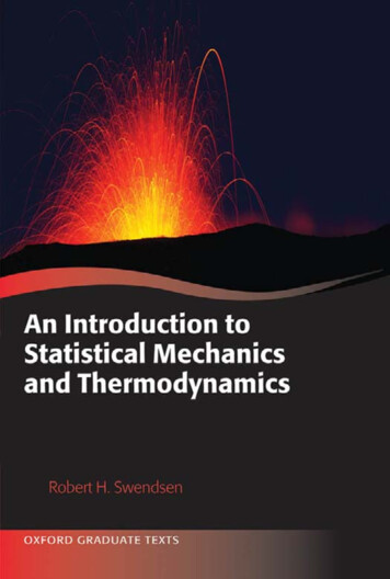
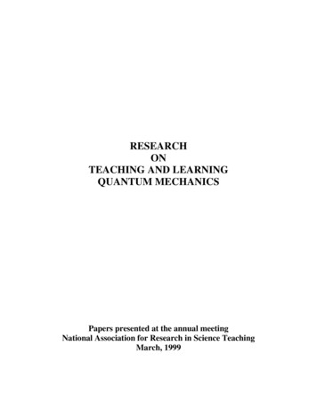
16M.O. ScullyFig. 2.1 Comparison of the quantum field, wave mechanical, and classical descriptions of the spin1 photon, spin 12 neutrino, and spin 0 meson; adapted from Scully and Zubairy “Quantum Optics”[3]Fig. 2.2 Top Down: The time-dependent Schrödinger wave equation follows from the quantumoptical “a photon is what a photodetector detects” definition. This is in accord with the usual wavefunction definition Ψ (r, t) r Ψ (t) since r Ψ̂ (r ) 0 . Bottom Up: The time-dependentSchrödinger wave follows nicely from the classical Maxwell equations by, for example, workingwith a combination of electric and magnetic fields2.2 The Quantum Optical Route to the Time-DependentSchrödinger EquationQuantum optics is an offshoot of quantum field theory in which we are often interested in intense light beams such as provided by the laser. However the issue of thephoton concept, and how we should think of the “photon,” is a topic of current andreoccurring discussion.Perhaps the most logical, at least the most operational, approach is to say that thephoton is what a photodetector detects. In this spirit we consider the excitation of a

2 Time Dependent Schrödinger Equation17single atom at point r at time t to be our photodetector and, following [3], write theprobability of exciting the atom as PΨ (r, t) η Ψ Ê † (r, t) Ê(r, t) Ψ .(2.1)Several points should be made:1. We consider the state Ψ to be a single photon state. For example, the stategenerated by the emission of a single photon (see [3], Eq. 6.3.18) ψγ ck k ,(2.2)k†where the state k is expressed in terms of the radiation creation operator âk as k âk† 0 and in the simple case of a scalar photon, we findck gke ik·r0,(νk ω0 ) iΓ /2(2.3)where gk is the atom-field coupling constant, r0 is the atomic position vector, νkand ω0 are the photon and atomic frequencies, and Γ is the atomic decay rate.2. The uninteresting photodetection efficiency constant η will be ignored in thefollowing.3. Ê † (r, t) and Ê(r, t) are the creation and annihilation operators defined byÊ † (r, t) † iνk t ik·rε(λ),k Ek âk,λ e(2.4)k,λwhere ελk is the unit vector for light having polarization λ and wave vector k,νk ck c k and the electric field “per photon” Ek νk /2ε0 V , where weuse MKS units so that ε0 μ0 1/c2 and V is the quantization volume. Next we insert a sum over a complete set of states, n n n 1 in Eq. (2.1) andnote that since there is only one photon in ψγ (and Ê(r, t) annihilates it), only thevacuum term 0 0 will contribute. Hence we havePψγ (r, t) ψγ Ê † (r, t) 0 0 Ê(r, t) ψγ ,(2.5)and we are therefore led to define the single photon detection amplitude asΨE (r, t) 0 Ê(r, t) ψγ .(2.6)As shown in detail in Sect. 2.4, the one photon state ψγ yieldsΨE (r, t) ΔrEΘ t e i(t Δr/c)(ω iΓ /2) ,Δrc(2.7)

18M.O. Scullywhere E is a constant, Δr is the distance from the atom to the detector, and Θ(x) isthe usual step function. More generally we have νkâk,λ e iνk t ik·r ψγ .ε̂kλΨE (r, t) 0 Ê(r, t) ψγ 0 2ε V(2.8)0k,λThe field is sharply peaked about the frequency ω so that we may replace thefrequency νk as it appears in the square root factor by ω and write ωϕγ (r, t) ,2ε0ΨE (r, t) (2.9)whereϕγ (r, t) ε̂k(λ)k,λ e iνk t ik·r ψγ .0 âk,λ V (2.10)The complete “photon wave function” also involves the magnetic analog of theproceeding. To that end we writeΨH (r, t) 0 Ĥ (r, t) ψγ ,(2.11)where Ĥ (r, t) is the annihilation operator for the magnetic field which is given byĤ (r, t) kr,λk ε̂k(λ) νke iνk t ik·râk,λ ,2μ0V(2.12)and we introduce the notation ΨH (r, t) ωχγ (r, t) ,2μ0(2.13)where ke iνk t ik·r (λ) ψγ . ε̂k ak,λ χγ (r, t) 0 kV k,λ(2.14)Finally, we write ϕγ (r, t) and χγ (r, t) in matrix form as ϕxϕγ ϕ y ,ϕz χxχγ χ y ,χz(2.15)

2 Time Dependent Schrödinger Equation19in terms of which Maxwell equations may be written as i t ϕγχγ 0 cs · p cs · p0 ϕγχγ ,(2.16)where p i and 00 0sx 0 0 1 ,01 0 0 01sy 0 0 0 , 1 0 0 0 1 0sz 1 0 0 0 0 0(2.17)are the 3 3 matrices for the (spin 1) photon.Finally, we note the close correspondence with the two-component (spinneutrino, ϕphotonχphoton ϕneutrino ,χneutirno1)2 (2.18)and the Dirac equation for the neutrino i t ϕνχν 0 cσ · p cσ · p0 ϕν,χν(2.19)where σ is given in terms of the 2 2 Pauli matrices and p i .We conclude by noting that, just as in the quantum field theory [4, 5] route tothe Schrödinger equation, the appearance of t and in Eq. (2.16) has not arisenfrom operator arguments. In the next sections, we follow a de Broglie wave–particleduality path to the Schrödinger equation.2.3 The Classical Maxwell Route to the Schrödinger EquationIn the previous section, we followed a top-down quantum field route to theSchrödinger equation, see Fig. 2.2. In particular, we saw that the quantum optical analysis of the single photon wave equation provided an interesting connectionbetween the Schrödinger (Dirac) equations for photons and neutrinos.In the present section, we start with the classical Maxwell equations and obtaina Schrödinger equation for the combination E iH which previous workers [6, 7]call the photon wave function. It is then natural to follow de Broglie and associate awave function with matter waves. This provides another (operator-free) route to theSchrödinger equation.

20M.O. ScullyThus, we define the “classical” photon wave function as ψx (r, t)Ψm (r, t) E(r, t) iH(r, t) ψ y (r, t) ,ψz (r, t)(2.20)where the subscript m stands for Maxwell. Along the lines of the discussion inSect. 2.2, we may write the Maxwell equations asi Ψ̇m (r, t) cs · pΨm (r, t) ,(2.21)where p i , as before, but now 00 0sx 0 0 i ,0i 0 0 0isy 0 0 0 , i 0 0 0 i 0sz i 0 0 .0 0 0(2.22)The present s matrix is related to the s of Sect. 2.2 by the factor i. It also should benoted that the present photon wave function ψm is a 1 3 matrix whereas that of 2.2is a 1 6 matrix. That is, the quantum optical analysis involves a two-componentwave function in Ψε and ΨH ; in the present analysis we find it convenient to combinethe electric and magnetic contributions at the outset.Since the energy per photon is ω ck cp, we writei Ψ̇m (r, t) H Ψm (r, t) ,(2.23)where the Hamiltonian is given byH cs · p .(2.24)The natural extension of this Schrödinger equation for the spin one masslessphotonto the case of a spin zero particle of mass m is clear. That is, since E 2 4m 0 c p 2 c2 is the finite mass extension of E pc, we follow the lead of deBroglie and writei Ψ̇ (r, t) m 20 c4 p 2 c2 Ψ (r, t) ,where p i , just as it is for the photon.Hence when m 0 c2havepc we may writei Ψ̇ (r, t) m 20 c4 p 2 c2 2 2 Ψ (r, t) ,2m 0(2.25)p22m m 0 c2 , and we(2.26)

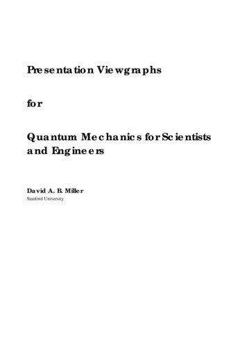
2 Time Dependent Schrödinger Equation21which is the non-relativistic wave equation, again obtained without introducingoperator-valued time or momentum.2.4 The Single Photon and Two Photon Wave FunctionsThe photon wave function concept really comes into its own when solving problemsinvolving photon–photon correlations. Then, as is explained in [8], the two photonwave functionψ (2) (r1 , t1 ; r2 , t2 ) 0 Ê(r2 , t2 ) Ê(r1 , t1 ) Ψ (2.27)is the subject of interest. Under some conditions this may be written in terms ofsingle photon wave functions, as in the case of two photon cascade discussed below.Some of the calculational details will be given since the physics (and the devil) is inthe details.Consider first the single photon wave function. From Eqs. (2.3) and (2.4) andignoring polarization, we find 0 Ê(r, t) ψγ 1.(νk )1/2 gk e iνk t eik·(r r0 )2ε0 V k(νk ω) iΓ /2(2.28)We now evaluate this function by converting the sum into an integral. The φ- and θ integrations can be carried out by choosing a coordinate system in which the vectorr r0 points along the z-axis. We then carry out the integration over k by evaluatingthe density of states and matrix elements at resonance. We are left with the integral dνke iνk t iνk Δr/c,(νk ω) iΓ /2which is evaluated via contour methods and where Δr r r0 is the distancefrom the atom located at position r0 to the detector. For t Δr/c, the contour liesin the upper half-plane and if t Δr/c, in the lower half-plane. On performing theintegration, we find ΔrEΔr 0 Ê(r, t) ψγ Θ t e i(t c )(ω iΓ /2) ,Δrc(2.29)where Θ is a unit step function and E is an overall constant with the units of electricfield.Next we consider the problem of “interrupted” emission, see Fig. 2.3. The firstphoton, associated with the a b transition, is described in the long time limit byour “old friend”