Transcription
Multi-Scale Pyramidal Pooling Network forGeneric Steel Defect ClassificationJonathan Masci and Ueli Meier and Gabriel Fricout and Jürgen SchmidhuberAbstract— We introduce a Multi-Scale Pyramidal PoolingNetwork tailored to generic steel defect classification, featuringa novel pyramidal pooling layer at multiple scales and a novelencoding layer. Thanks to the former, the network does notrequire all images of a given classification task to be of equalsize. The latter narrows the gap to bag-of-features approaches.On various benchmark datasets, we evaluate and compare oursystem to convolutional neural networks and state-of-the-artcomputer vision methods. We also present results on a realindustrial steel defect classification problem, where existingarchitectures are not applicable as they require equally sizedinput images. Our method substantially outperforms previousmethods based on engineered features. It can be seen as a fullysupervised hierarchical bag-of-features extension that is trainedonline and can be fine-tuned for any given task.I. I NTRODUCTIONAutomated Inspection Systems in steel industry aim atrecognizing material defects to improve product quality andreduce production costs and human intervention. This isperhaps one of the most crucial phases of the whole qualitycontrol pipeline. Over the years, many efforts have beendevoted to crafting features to solve this problem. Latestadvances in technology suggests new acquisition systems(such as high-resolution and hyper-spectral cameras), makingconventional features perform poorly. Handcrafting a new setof features plus corresponding parameters is a cumbersomeprocess which may cost several man years and lots of money.It might be virtually impossible where the engineers havelittle prior knowledge, e.g., in the case of hyper-spectralacquisitions.It is then paramount to have a self-adjusting system requiring only minimal efforts for manual selection of parameters.This issue is addressed widely in the literature. Below webriefly review the best frameworks in computer vision (CV)and machine learning (ML), respectively.Many CV systems adopt the bag-of-features (BoF) approach [1]. For a given image a set of features (e.g.SIFT descriptors [2]) are extracted and then encoded inan overcomplete sparse representation using a dictionarybased technique. This produces a histogram of “active”words representative of the content of the image. The featureextraction is hard-coded whereas the dictionary is specificallybuilt for a given task. That is, for classification tasks featurevectors from all or a subset of images from the training setare collected and clustered. The cluster centers form the basisJonathan Masci and Ueli Meier and Jürgen Schmidhuber are with IDSIA,USI and SUPSI Galleria 2, 6928 Manno-Lugano, Switzerland {jonathan,ueli, juergen}@idsia.ch Gabriel Fricout is with Arcelor Mittal MaizièresResearch SA, France {gabriel.fricout@arcelormittal.com}Jonathan Masci was supported by ArcelorMittal.of the dictionary that is used in the coding stage. Finallya supervised classifier is trained to classify the histogramrepresentation of the image. This approach does not discovernew and possibly very discriminative features and usesconventional algorithms. The effort is all in the encodingstage where a per-task dictionary of words is learned.Supervised ML methods, on the other hand, try to mapthe pixel-based representation directly into a label vector,learning both feature extraction and encoding from a labelleddataset. Learning the features from the data helps to make thesystem easily applicable to domains where prior knowledgeis not well consolidated, in particular in the case of texturedsteel, where the distinction between acceptable and defectpatterns is hard even for the most advanced and consolidatedsystems. Perhaps the most successful methods for imageclassification are variants of Convolutional Neural Networks[3], [4], [5], [6] (CNN) reminiscent of simple and complexcells in the primary visual cortex [7]. Learning good featureswith such models, especially in cases where the numberof training samples is scarce, opened up the investigationof unsupervised algorithms which can be used as a pretraining stage. This approach has become quite popularand is widely used [8], [9], [10], [11] to obtain betterfeature extractors in such setups. Whether pre-training leadsto improved recognition accuracy for classification tasks isquestionable though [12]. As long as a labelled dataset isavailable, fully supervised approaches seems to be preferablein many benchmarks [13]. For handwritten characters, elasticdistortions and deformations are the best way to avoid overfitting and improve generalization [14], [15], [13]. CNN havebeen recently shown [16] to outperform any conventionalfeature for the task of steel defect classification, the onlymajor limitation being the partitioning and resizing of thedata to fit the constraint on equally sized input images. Thisrequires several networks to be trained on a subset of thedata, which reduces considerably the number of trainingpatterns per class and makes training almost impossible indomains where labelled data are expensive, requiring thensystems able to learn just from few samples per class.Furthermore, the desired invariances for general steel defectrecognition are not that easily synthesized—most of thedefects cannot be detected by rotation invariant descriptors,and in most cases the scale is of crucial importance, too. Adistortion/deformation-free approach is preferable.There are obvious similarities between BoF and fullysupervised CNN. Both extract features based on photometricdiscontinuities (e.g., edges), either engineered or learnedfrom samples followed by an encoding stage. Standard CNN
lack multiple resolution pooling and the explicit encodingsteps of winning BoF approaches. BoF, however, lack tunablefeature extraction stages that may make complex encodingsless important. A main drawback of CNN is their restrictionto constant size input images, which the steel industry cannotsimply overcome by resizing and padding.A. ContributionsHere we present the MSPyrPool framework which aimsat solving the general steel defect recognition problem. Wefurther close the gap between BoF and CNN by introducingan extension of commonly used convolution-based nets forthe steel industry, consisting of three new ingredients: a back-propagation-compatible Pyramidal Pooling layerwhich produces a fixed-dimensional feature vector independent of the input image size; a learnable encoding layer to incorporate commonlyused encoding strategies of CV; a Multi-Scale feature extraction strategy.Our approach is the first applicable to general steel defectclassification problems with arbitrarily sized images. It scalesstraightforwardly to multi-variate (hyper-spectral) images,the coming standard in automatic steel inspection.II. R ELATED W ORKSObject recognition algorithms usually use the followingscheme: feature extraction, encoding, classification. In CVis desirable to obtain a linearly separable code that canbe effectively classified with a linear SVM for scalabilityreasons. This does not affect ML methods as the predictioncomes at a linear cost of the forward pass of the network.In what follows we briefly recall first the CNN generalarchitecture and then the two main concepts of a BoF systemwhich will be reinterpreted in our MSPyrPool architecture.A. Convolutional Neural NetworksCNN are hierarchical models alternating two basic operations, convolution and subsampling, reminiscent of simpleand complex cells in the primary visual cortex [7]. Theyexploit the 2D structure of images via weight sharing, learning a set of convolutional filters. This powerful characteristicmakes them excel in many object recognition [17], [6],[15], [16] and segmentation [18], [19] benchmarks. CNN arecomposed of the following layers: Convolutional Layer: convolves the set of input images{fi }i I with a bank of filters {wk }k K , producinganother set of images {hj }j J denoted as maps. Aconnection table CT specifies input-output correspondences (inputImage i, filterId k, outputImage j). Filterresponses from inputs connected to the same outputimage are linearly combined. This layer performs thefollowing mapping:Xhj (x) (fi wk )(x),(1)i,k CTi,k,jwhere indicates the 2D valid convolution. Each filterwk of a particular layer has the same size and defines,together with the size of the input, the size of the outputmaps hj .The output maps are passed through a nonlinear activation function (e.g., tanh, logistic, etc.). Pooling Layer: down-samples the input images by aconstant factor keeping a value (e.g. maximum or average) for every non overlapping subregion of size pin the images. This layer does not only reduce thecomputational burden, but more importantly performsfeature selection. Fully Connected Layer: this is the standard layer of amulti-layer network. It performs a linear multiplicationof the input vector by a weight matrix.Max-Pooling is our favored type of pooling, as it introduces invariances to small translations and distortions, andleads to faster convergence and better generalization [20].The corresponding CNN are called Max-Pooling CNN,MPCNN for short. They are, so far, the best choice for awide array of applications [17], [6], [15], [16].B. Feature Encoding AlgorithmsIn the CV framework, features are extracted using engineered approaches (e.g. SIFT descriptor). What usuallyvaries is not the feature extraction procedure but where inthe image to extract the descriptors. The most successfulmethods extract features over a dense, equally spaced grid[21]. Recent improvements in classification performance oncommonly used benchmarks [22] are rather due to improvedencoding strategies than new feature descriptors. In order toproduce a histogram, the descriptors need to be quantizedsuch that they can be matched against a given codebook.This step is crucial to produce encodings with the rightlevel of detail that avoids overfitting and leads to improvedgeneralization to unseen data. The de-facto standard for thisprocedure seems to be given by overcomplete and sparseencodings of the feature descriptors. Most commonly usedalgorithms for this step are: Vector Quantization (VQ) whereonly one basis is selected; Sparse Coding (SC) where a smallsubset is kept; Locality-constrained Linear Coding (LLC)where the subset of basis, of fixed size, is selected usingK-NN leading in fast coefficients estimation solving a verysmall least-squares problem.C. Feature PoolingOnce the features are encoded a histogram is formed. Thenaı̈ve approach, used in early BoF systems, is to sum allthe N -dimensional codes, where N represents the numberof bases in the dictionary, thus producing a global representation. A more powerful histogram generation techniqueis presented in [23], where features are considered in theirspatial locality. At every level l of a quad-tree 2l tiles areproduced and for each tile a feature vector is extracted.This approach is used in the PHOG descriptor [21], animprovement over HOG [24]. In conjunction several methodsto pool have been presented, such as sum-, average-, and 2 pooling.
III. M ULTI -S CALE P YRAMIDAL P OOLING N ETWORKCNN and BoF approaches share many building blocks.Both extracts features using convolutional filters, with theonly difference being that the filters of a CNN are learnedfrom the data whereas fixed feature extractors are used inBoF. Furthermore, BoF is inherently single layer, whereasdeep multilayer architectures are capable of extracting morepowerful features [25]. For HOG the image gradient isobtained using convolutional filters and then pooled to obtainthe final descriptor. In SIFT an input patch of 64 64 pixelsis tiled in 16 quadrants and for each of them a 8-dimensionalvector of gradient orientation is extracted. The resultingdescriptor is a concatenation of such vectors resulting in a128-dimensional feature vector positioned at the centre ofthe input patch. If we interpret a CNN as a composition ofmany functions (e.g. layers), we obtainCN N (x) fc . . . fk . . . fe . . . f1 (x),(2)2 2; this clearly equals to a Pyramidal Pooling with 5 tilesin each dimension.The Pyramidal Pooling layer does not have any tunableparameters but in order to train the feature extraction layersbefore it the partial derivative of the layer’s output w.r.t. itsinput is required. Let us denote by X the 3-dimensional inputvector of images (e.g. [#rows, #cols, #maps]). During theforward pass max-pooling keeps only the maxima valuesin non overlapping sub-regions of X, down-sampling theimages by a constant factor. The backward pass places thedelta values (results of partial differentiation by applying thechain-rule) at the location at which the maxima was found,up-sampling to the original input size. In our pyramidalpooling layer the forward pass is equivalent to applying asubsampling operation at each level of the pyramid and thenconcatenating the result into a single output vector. Consequently the backward pass sums over the back propagationof each of the pyramid levels.where f1 to fe represent the feature extraction layers, fe to fkthe encoding layers and fc the remaining classification layers.Providing a differentiable definition for each layer results ina framework whose parameters can be jointly learned froma labeled training dataset. In what follows we introduce twonew layers that are used in our MSPyrPool framework.A. Pyramidal Pooling LayerIn previous work [26] a dynamic pooling layer is usedto obtain features independent of input size, to detect paraphrases of 1D signals. Here we present a variation whichtakes into account the 2D nature of images and producesspatially located representations at several resolutions following [23]. Let us consider a layer with k maps, each mapcorresponding to a filtered/pooled image. If all the values ineach of those maps are summed, a k-dimensional featurevector which does not depend on the actual input imagesize, is obtained. This produces a representation that onlydepends on the number of maps producing a system which nolonger requires fixed size images. This already represents amajor improvement to obtain a generic steel defects classifier.However, summing all the activations of a map results inhigher values for bigger images. To obtain a more stablemeasure, average pooling is usually preferred. An even moreeffective way of performing feature pooling uses the maxoperator instead of the average. This avoids normalization alltogether and in our experiments always speeded up learning.Hereafter we consider only pyramidal pooling layers withmax-pooling.To produce a spatially localized feature vector we dividethe image in tiles and pool over the quadrants varying thepooling window accordingly. The final representation is thenobtained concatenating the results of each of the levels,just as in BoF and is schematized in Figure 2. Using asufficient number of tiles Pyramidal Pooling is equivalent tothe conventional pooling operation of CNN and can thereforebe considered as its generalization. Let us for exampleconsider the case of 10 10 images and max-pooling of.L1L2Fig. 2. Pyramidal Pooling Layer. Features are pooled along l2 equallysized quadrants and the histogram-like representations are concatenated toform a feature vector.B. Multi-scale extractionA pyramidal feature extraction, while being itself alreadyan improvement over conventional CNN, as it allows torelax the constraint on a fixed input size, extracts featurescorresponding only to a single scale (e.g. the nominal sizeof the “simplified” image where the pooling is performed).In many applications, where input images come at verydifferent scales, applying a pyramidal pooling layer willnot completely solve the problem. Multi-Scale pyramidalfeature extraction can be done using a pyramidal poolinglayer for each representation (i.e. layer in the network),and then concatenating the various feature vectors for theclassification stage. After a subsampling layer the image getsdown-sampled by a constant factor and attaching a pyramidalpooling before and after a max-pooling operation thereforedelivers a Multi-Scale feature extraction (Fig. 1).
ConvolutionPoolingL1L2Pyramidal PoolingL1MLPPredictionL2Fig. 1. Schematic representation of a MSPyrPool Network where histogram-like representations are extracted at two levels and at two scales. The firstscale represents the output of the convolutional layer whereas the second scale is given by the output of a pooling (downsampling) layer. The resultingfeatures are concatenated and used as input for the classification layer.C. Feature encoding layerThe next step in narrowing the gap between the conventional BoF approach and CNN is represented by introducinga feature encoding layer, the major contribution of thiswork. If we consider the simplest of the feature quantizationalgorithms of BoF, k-means with hard assignment, we notethat such an algorithm can be approximated by a correlationbased measure 1 . This allows us to derive a differentiableapproximation of such coding scheme which we name asMLPDict.1) MLPDict Layer: We use a fully connected layer withmax-pooling to mimic the behavior of k-means coding. Theprojection of x with W, the weights of the encoding layer, isthe correlation between x and each column of W. Taking themaximum approximates the VQ coding scheme. Comparedto the BoF approach, W serves as the dictionary, however anadaptive one which is tuned sample after sample. Performinga pyramidal pooling operation on the result of such anencoding will produce a histogram-like representation.Figure 3 shows a schematic representation of the encodinglayer. The hidden representation of a convolutional-basednetwork is composed of D images; we consider each pixel asa D dimensional feature vector (extracted from the densestgrid). MLPDict reshapes D into a matrix with as manyrows as pixels (#rows #cols) and as many columns asimages (#maps). Applying a fully connected MLP layer0with a weight matrix W RD D to the reshaped matrix0N D0X Rwill result in X RN D . This is reshaped0back onto D images, where N corresponds to the numberof pixels in each image. When D0 D it acts as afeature selection layer which reduces redundancies; commonstrategy in image processing, especially in hyper-spectraldata processing. When D0 D the layer, thanks to themax-pooling operation, acts as a conventional VQ encodinglayer. This is what we use in all our experiments; however theqPpPP 2P22 y 2 i (xi yi ) i xi i yi 2i xi yi ,and in the case of x and y normalized to have zero mean and unit variancereduces to the correlation between x and y as their sum will be almostconstant.1 xapproach is general and extendible to any feature encodingalgorithm.IV. E XPERIMENTSIn all experiments, unless stated otherwise, we evaluatethe average per-class accuracy to establish the classification performance, a more meaningful measure in case ofunevenly distributed datasets. No additional preprocessing,such as translation or deformation is used because of theaforementioned requirements of steel industry. Of course anyad-hoc transformation of the data can be easily plugged into improve performance. All nets are trained using stochasticgradient descent (mini-batch of 1) with initial learning rateof 0.001, annealed by a factor of 0.97 at every epoch andmomentum term of 0.9. Best results are usually reached infew training epochs ( 30), whereas for CNN many moreare generally required, especially when transformations areadded to the input. Softmax activation is used at the outputlayer and the Multi-Class Cross-Entropy loss is minimized.We validate our model first on publicly available benchmarksto compare with other published approaches. We then showresults on a challenging dataset from the steel industry whereour MSPyrPool framework can be applied directly and whereCNN fail.Comparing our architecture with CNN is not an easy taskas the two approaches differ considerably. Nevertheless wetry to make the comparison as fair as possible by takingequally sized convolutional and subsampling layers in botharchitectures and letting them differ for the choice of theencoding and classification stages. The two systems equalsfor a particular choice of the MSPyrPool parametrization.GPU Implementation The proposed framework requireslot of computational resources to train. We provide a GPUimplementation using Arrayfire [27] for which we experienced speed-ups in the range 15 40 , without loosingflexibility and ease of coding.A. Conventional BenchmarksWe select three common evaluation datasets: digit, textureand object recognition. All of them belong to quite orthogo-
D’D’f(x).#pixelsD#pixelsDfeature encoding(MLPdict, LLC, .)Fig. 3. The MLPdict layer used for feature encoding. Image responses of a network layer are reshaped to produce D dimensional feature vectors, whereD represents the number of images in the layer. Each pixel descriptor is mapped into another representation of size D0 for which only the maxima valueper row is preserved.nal domains for which ad-hoc techniques are usually applied.In particular the latter one shows clearly the advantage of aMSPyrPool network w.r.t. CNN in the context of fully supervised classification. No particular tuning of the architecturehas been made as the aim of this section is to show therelative improvement of MSPyrPool nets over CNN.1) MNIST: As a reference to compare our approach witha conventional CNN we take the well studied MNIST [4]benchmark of handwritten characters. CNN excel on thisdataset where all digits are of equal size and centered in themiddle of a 28 28 grey-scale image. For this experiment theoverall classification accuracy is used to easily compare withother methods. We use a MSPyrPool net with a convolutionallayer with 5 5 filters and 100 output maps (C 5 5 100),a 2 2 max-subsampling layer (MP 2 2), a pyramidalpooling with linear MLPDict at the output of the twosubsampling layers with l {1, 2, 4, 8} and l {1, 2, 4}quadrants respectively. Results are shown in Table I. It isinteresting to note that our approach is the best among thefully supervised CNN approaches and on-par with the oneswhich use unsupervised pre-training while just using a verysmall single layer network and 100 filters.TABLE IC LASSIFICATION RESULTS FOR THE MNIST BENCHMARK . O URMSP YR P OOL NETWORK IS COMPARED WITH OTHER CNN- BASEDAPPROACHES WHICH DO NOT USE ANY INPUT PREPROCESSING .CNN LeNet-5 [4]CNN pre-training [28]CNN pre-training [11]MSPyrPoolTest %99.0599.4099.2999.132) CUReT: The Columbia-Utrecht (CUReT) database[29] contains 61 textures; each with 205 images obtainedunder different viewing and illumination conditions. Fortraining our architecture only a single image is required asinput, just as in previous work [30], with no information(implicit or explicit) about the illumination and viewingconditions. We use the conventional evaluation protocol [30]but with a different random split of the data. Images are normalized to have zero mean and unit variance to compensatefor very different light conditions. We train a CNN with 5hidden layers: C 11 11 20, MP 5 5, C 9 9 20, MP5 5, classification layer. We use tanh as activation for everyconvolutional layer. We compare the result with a MSPyrPoolwith tanh pyramidal pooling MLPDict and codebook size of100 at the output of the first and second convolutional layers,keeping the rest of the network topology. Features are pooledusing l {1, 2, 4} and l {1, 2, 3} levels producing a 3500dimensional vector.Table II compares our new MSPyrPool network withconventional CNN. The MSPyrPool net generalizes muchbetter to the unseen test data and shows the superiorityover conventional CNN for the task of texture classification,a domain closely related to steel classification. We alsoreport results for the case where no MLPDict is used, tofurther show that the encoding stage is important and deliversindeed non-marginal improvements in final classificationperformance. The approach reaches 99.0% recognition rateon all 61 classes and thus greatly outperforms bank-of-filterand Texton (96.4% [30]), whose similar architecture has prewired feature extractors. So the novel layers help indeed tolearn better features, and are a valuable contribution to theCNN framework.TABLE IIC LASSIFICATION RESULTS FOR THE CUR E T BENCHMARK . ACONVENTIONAL CNN IS COMPARED WITH OUR MSP YR P OOLNETWORK .W E ALSO SHOW THE RELATIVE IMPROVEMENT OF AMLPD ICT ENCODING STAGE .Textons [30]CNNMSPyrPool (no encoding)MSPyrPoolTest %96.496.593.899.03) Caltech101: A further validation of the proposed system is performed on a classical pattern recognition benchmark, Caltech101, where fully supervised CNN have seldomly successfully been applied. Usually ad–hoc prepro-
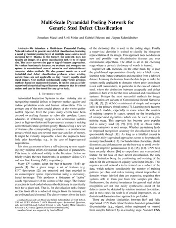
cessing stages and tailored non–linearities are required toobtain a satisfactory performance. We compare our resultswith those obtained with the similar system which usesconventional BoF with VQ [23]. We use 30 images per classfor training and we test on at most 50 of the remainingimages converted to grey-scale. We consider a net with andwithout an encoding layer. Both nets are composed by: C16 16 100, MP 5 5. For the net without an encodinglayer a pyramidal pooling layer with l {1, 2, 4} is usedto create a 2100-dim feature vector. For the net with anencoding layer, we used a dictionary size of 1024 just beforethe pyramidal pooling layer. Using a pyramidal pooling layerwith l {1, 2, 4} results in a 21504-dim feature vector.We train both a net with a linear and non-linear activationfunction in the encoding layer. For the sake of completenesswe also train a CNN consisting of: C 16 16 100; MP 5 5;C 13 13 100; MP 5 5; fully connected classification layer.This CNN architecture is by no means the best architecturefor this task, and is only listed to quantify the improvementusing MSPyrPool nets. Results of all experiments togetherwith results from the literature are listed in Table III.In this context the established industrial pipeline involvesa series of hand-crafted features which are hard to selectand tune. This is particularly true for multi-variate imageswhere prior knowledge is still not consolidated to producean effective way of extracting steel features.In [16] the authors show that features can be effectivelyand efficiently learned from raw-pixel intensities of steeldefects using CNN, delivering online processing times andsuperior performance. Their approach inherits all the benefitsof CNN and therefore extends well to any kind of inputimages and does not require any prior knowledge on the task.Unfortunately the intra-class defect variability makes the taskof dividing the images into homogeneous size/ratio clusterscumbersome (defects within the same class can appear atvery different sizes). The number of available samples fortraining would reduce dramatically. Using a MSPyrPool netavoids such problems because of the input-size independentfeature extraction, one of the main contributions of this work,and makes convolution based networks applicable to thegeneral steel defect recognition task for the first time. ForTABLE IIIC LASSIFICATION RESULTS FOR THE C ALTECH 101 BENCHMARK . AMSP YR P OOL NET WITHOUT AN ENCODING LAYER ( NET 1), WITH ALINEAR ( NET 2) AND A NONLINEAR ENCODING LAYER ( NET 3) ARELISTED .CNNnet1net2net3Spatial Pyramid [23]LLC [22]Test %25.252.858.055.264.673.4MSPyrPool nets clearly improve recognition rate compared to a similar sized CNN.2 Using an encoding layerimproves generalization performance even though the resulting nets have many more free parameters. Results showthat we are able to jointly learn the feature extraction, thequantization and the classification stages fully online in aparticularly difficult domain where unsupervised pre-trainingis required in most ML systems. We also see that theencoding stage does not match the performance of the CVsystem, perhaps due to the single layer architecture adoptedto mimic the one of SIFT descriptors.B. Steel-Defects Industrial BenchmarkSteel is a textured material and defects come at varyingscales, which makes the task of classifying a wide range ofdefects extremely difficult. It is not easy to find a good resizing technique without destroying the original informationcontent of the images. As a matter of fact if images/objectsin a given classification task are varying over a few order ofmagnitudes it is even impossible to resize or pad the images.2 Better results are obtained with deeper and bigger CNN, we got 40%with a huge CNN still worse than MSPyrPool.Fig. 4. Subset of images from the Steel-defects benchmark showing thegreat difference in size among various samples. In this setting is not possibleto resize the images to the same size, hence a CNN is not applicable to solvethis task.this experiment we use a proprietary dataset of ArcelorMittalfrom a hot-strip mill production line containing 30 differentdefect classes. A region-of-interest (ROI) is provided for eachof the instances which vary greatly in size from a minimumedge length of 20 to a maximum of 2000 pixels(Fig. 4). Furthermore the dataset is unevenly distributedw.r.t. the number of samples per class; a task where thefull potential of our model can be appreciated. To obtaina good support to perform the pyramidal pooling we addbackground information to get a minimum patch size of 100pixels along each dimension whenever possible and zero-padotherwise. We also limit the maximum size per dimensionto 500 pixels to accelerate training. We compare our systemto a set of classifiers trained on commonly used featuresusing the same evaluation protocol described in [16] butwith a larger MLP for classification (500 units) as the task
Fig. 5.Two misclassified images for which the network inverted thecorresponding classes (off diago
Once the features are encoded a histogram is formed. The na ıve approach, used in early BoF systems, is to sum all the N-dimensional codes, where represents the number of bases in the dictionary, thus producing a global repre-sentation. A more powerful histogram generation technique is presented in [23], where features are considered in their