WIXLIB

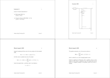
Standard LMSLecture 41u(n)-DatavektorM 12u(n)rb T (n)u(n)y(n) w- m1 1ry(n)-6rbw(n)Lecture 4 contains descriptions ofM 1Delayb 1) 6w(n m Block-based LMS (7.1)(edition 3: 10.1)6 mrµ6 Frequency Domain LMS (FDAF, 7.2-7.3)(edition 3: 10.2-10.3)b J(n) u(n)e(n)–? e(n)- m Σ 6 d(n)Adaptive Signal Processing 2011Lecture 4Block-based LMS3Instead of updating the filter vector for every sample as for the standardLMS, 4The gradient estimation can in this case be written asL 1X u(kL i)e (kL i) ,i 0the filter vector is updated once every lth sampel,b (k 1) wb (k) µwLecture 4Block-based LMSΦ(k) b (n 1) wb (n) µu(n)e (n) ,wL 1XAdaptive Signal Processing 2011which is referred to as a time averaged gradient vector. u(kL i)e (kL i) ,i 0where the sample index n and block index k are related asInstead of updating the filtervector with a gradient vector at everysample, the filter vector is updated for every Lth sample with the sum(which is a weighted average) of the gradient vectors for the last Lsamples.n kL i .Adaptive Signal Processing 2011Lecture 4Adaptive Signal Processing 2011Lecture 4

Block LMS51 Mu(n)-DatamatrisM Lu(k) } {zb T (k)u(k) [y(kM M 1), . . . , y(kM )]y(k) w r- m-rConvergence properties for the Block-LMS6rbw(k)Delay Both the LMS and the Block-LMS minimizes J(n) E{ e(n) 2}.b 1) 6w(k m6 m6M 1 Both the LMS and the Block-LMS converges towards the Wienersolution.rµ6 The Block-LMS uses a better estimate of the gradient. This will,however, not result is a faster convergence.b J(k) u(n)eT (n) e(k) [e(kM M 1), . . . , e(kM )]- m –? Σ 6 d(k) [d(kM M 1), . . . , d(kM )]Adaptive Signal Processing 2011Lecture 4Convergence properties for the Block-LMSAdaptive Signal Processing 20117Lecture 4Convergence properties for the Block-LMS8 The convergence criteria for the Block-LMS is 0 µ Lλ 2 .maxThe natural choice of the block length (L) is the filter length (M ). This upper limit for µ makes the Block-LMS converge slower thanthe LMS, especially for large eigenvalue spread.If L M the gradient estimation is based on more information thanthe filter If a block length of L is chosen to increase the calculations speed,the Block-LMS may become slower in converence speed because ofthe stricter limit of µ.If L M the entire filter is not used because not enough samples areincluded in the block. Misadjustment is the same as for the LMS.Adaptive Signal Processing 2011Lecture 4Adaptive Signal Processing 2011Lecture 4

Summary of the Block-LMS9Two strategies for reduction of the complexity10b T (k)u(kL i), L st1. y(kL i) wi.e.,b T (k)u(k).y(k) w1. Adaptive IIR filters can generate long impulse responses for few weights stability problems2. e(kL i) d(kL i) y(kL i)i.e.,e(k) d(k) y(k).2. Frequency Domain Adaptive Filters (FDAF). This strategy is based on the Block-LMS but the heavy calculations are made in thefrequency domain. These methods can also be used to improve theconvergence properties pof the LMS algorithm.PL 1b (k 1) wb (k) µ i 0u(kL i)e(kL i)3. wi.e.,b (k 1) wb (k) µ u (k)eT (k).w In applications with long filters, e.g. echo cancellation, the complexitybecomes very high. The equations that take time are the filtering in (1)and the cross correlation in (3).Adaptive Signal Processing 2011FDAFLecture 411In order to increase the calculation speed of the LMS algorithm, thefiltering (convolution) and the gradient estimation (crosscorrelation)can be done in the frequency domain instead of the time domain.Strategy:Adaptive Signal Processing 2011ProblemLecture 412Multiplication in the frequency domain corresponds to circular convolution, butr in order to maintain the properties of the LMS, linearconvolution must be used. Filtering must be done with linear convolution.1. FFT of input and error signals2. Convolution and crosscorrelation corresponds to multiplication inthe frequency domain Gradient estimation should be done with linear convolution. Thenthe method is called Fast LMS. If linear convolution is not usedhere the method is called Unconstrained FDAF.3. IFFTTwo advantages of the FDAF:1. Faster calculation2. Independent coefficientsAdaptive Signal Processing 2011Lecture 4Adaptive Signal Processing 2011Lecture 4

Fast LMS (FDAF med gradientvillkor) [u(k 1), u(k)]u(n)-Datavektor1 2M- FFTdiagrU(k)- mY(k)- IFFT y(k)13 -6rSparasista blocketry(k)-Properties of the Fast LMS14cW(k)Delay Fast LMS is based on the Block-LMS and converges similarly.c 1) 6W(k m6 m To calculate and update the filter in the frequency domain opensnew possibilities.rα6FFTUH (k) diag(FFT([uR (k), uR (k 1)]))6 Lägg till nollblock sist6 Spara förstablocketφ(k)0φ(k) In the LMS, each filter weight represents a mix of the differenteigenmodes. In the Fast LMS, each filter weight is directly connected to ascertain eigenmode (frequency range).6?( ) IFFT 6 mr D(k)0e(k)6- m E(k)FFT The filter weights of the FastLMS is therefore updated independently of each other. Lägg tillnollblock först e(k) ?– Σ 6 d(k) [d(kM ), . . . , d(kM M 1)]TAdaptive Signal Processing 2011Lecture 4Properties of the Fast LMS, cont.Adaptive Signal Processing 201115 The convergence speed for the Fast LMS can be optimized for eachmode separately. The convergence speed for the i:th mode depends on µλi. Ameasure of λi is the average power in the frequency bin of the i:thmode,Pi Ui 2 .If µi Pα , all modes will converge equally fast (WSS).i If the imput signal is not WSS, Pi must be estimated recursivelyPi(k) γPi (k 1) (1 γ) Ui(k) 2 The stepsize parameter µ is here substituted by a diagonal 2M 2M matrix µ αD(k), where D(k) 1diag[P0 1, P1 1, . . . , P2M 1 ].Adaptive Signal Processing 2011Lecture 4Lecture 4Fast LMS, Update equations16ˆ TU(k) diag(FFT u((k 1)M ). . .u(kM 1), u(kM ) . . .u((k 1)M 1) )c (k)]y(k) Last M elements of IFFT[U(k)Wˆd(k) d(kM )d(kM 1). Td((k 1)M 1)e(k) d(k) y(k)–»0E(k) FFTe(k)HP(k) γ P(k 1) (1 γ)U (k)U(k)h 1 1P1 1 (k)D(k) P(k) diag P0 (k).P 1(k)2M 1iHφ(k) First M elements of IFFT[D(k)U (k)E(k)]–»c(k 1) Wc (k) αFFT φ(k)W0Adaptive Signal Processing 2011Lecture 4

FDAF utan gradientvillkor18 [u(k 1), u(k)]Unconstrained FDAF17u(n)-Datavektor1 2M- FFTdiagrU(k)- mY(k)- IFFT y(k) -6rSparasista blocketry(k)-cW(k)Delay Three out of the five FFT/IFFT operations in the Fast LMS is usedto perform the filtering with linear convolution (required).c 1) 6W(k m6 m Two out of the five FFT/IFFT operation in the Fast LMS is usedto perform the gradient estimation with linear convolution. This iscalled the time-domain constraint.c(k 1) Wc (k) µUH (k)E(k)WUH (k) diag(FFT([uR (k), uR (k 1)])) FDAF can be used without satisfying this constraint, i.e., withgradient estimation based on circular convolution. Then the updateequeation becomesrα6?( ) - m E(k)0e(k)FFT Lägg tillnollblock först e(k) ?– Σ 6 d(k) [d(kM ), . . . , d(kM M 1)]TAdaptive Signal Processing 2011Properties of the Unconstrained FDAFLecture 419 Does not converge towards the Wiener solution.Adaptive Signal Processing 2011Suggested readingLecture 420 Haykin chap. 7 (7.4-7.6 for extra depth)edition 3: 10 (10.4-10.6 for extra depth) Larger misadjustment. Poorer gradient estimation results in twice as many iterations inorder to reach the same misadjustment as the Fast LMS.Computer exercise theme: Apply FastLMS to echo cancellation of speechsignal. Faster calculations.Adaptive Signal Processing 2011Exercises: Haykin exercise 7.2, edition 3: 10.2Lecture 4Adaptive Signal Processing 2011Lecture 4

Adaptive Signal Processing 2011 Lecture 4 6 Both the LMS and the Block-LMS minimizes J (n) E fj e (n) j 2 g. Both the LMS and the Block-LMS converges towards the Wiener solution. The Block-LMS uses a better estimate of the gradient. This wi ll, however, not result is a faster convergence. Adaptive Signal Processing 2011 Lecture 4 Convergence .