Transcription
Harvard-MIT Division of Health Sciences and TechnologyHST.584J: Magnetic Resonance Analytic, Biochemical, and Imaging Techniques, Spring 2006Course Directors: Dr. Bruce Rosen and Dr. Lawrence WaldMR Image EncodingL. Wald MGH-NMR CenterMR Image EncodingIntroductionMuch of the success and flexibility of MRI is derived by its peculiar methodology; a setof techniques which has proved to be very flexible and informative for probing the properties ofcomplex materials (such as the brain). MR imaging is fundamentally different from other typesof imaging. Conventionally, when physicists refer to “imaging” they refer to a scatteringexperiment. Since our eyes “see” a rock by forming a 2 dimensional array of light intensityamplitudes being scattered off the rock, the instrumental equivalent of this has come to besynonymous with imaging. In the canonical scattering experiment, “rays” are aimed at an objectand then detected as they either scatter off of the object or penetrate through it. The rays can bedeflected, lose or gain energy, deflect and then interfere with one another or even be convertedfrom one type of ray to another. The “rays” in question are usually electromagnetic radiation(radio waves, microwaves infra red light, visible light, ultraviolet light, x-rays, or gamma rays)but can, of course, be almost anything including sound waves, water waves, or matter waves(particles). The particles used could be electrons (as in electron microscopy), or any of thezillions of other subatomic particles, or clumps of particles such as nuclei, atoms, molecules, orpieces of dirt.A fundamental limitation of scattering experiments is that the resolution of the imagecannot exceed the wavelength of the wave (electromagnetic or matter wave) used to probe theobject. This is fundamentally derived from the uncertainty principle but has long beenunderstood in classical optics. Physicists are fond of making such general statements, but,while true for scattering experiments, this imaging “law” does not hold for MRI. In MR, we useradio waves with a wavelength of several meters to image at a sub-millimeter resolution. Thuswe exceed this “fundamental” imaging law by several orders of magnitude. How? The shortanswer is that we don’t determine the distribution of the body’s protons by bouncing stuff off ofthem; we determine it by asking them to report to us where they are. We query the body’s spinsusing a burst of radio waves (the excitation RF), and they report back some milliseconds laterwith a faint radio signal of their own. They declare their location and other even more valuableinformation encoded in the frequency and phase of the burst of RF energy they emit in response(the MR signal or echo).MR Image EncodingReview of the basic NMR experimentThe previous lectures reviewed the basic equationsof motions of the proton spin placed in a static, uniform magnetic field. The state of a givenspin is either parallel or anti-parallel to the static field. Since the parallel state is slightlyenergetically more favorable, a slim majority are found in this state. When the vector sum of allof the spins is considered, there is almost a complete cancellation between the aligned and antialigned spins; the net magnetization consists of the only the slight excess aligned with themagnetic field. Since the other spins always have a canceling partner, we do not detect themand only the small ( 0.01%) excess aligned magnetization, Mo, will be considered. Althoughquantum mechanics tells us that a measurement of the energy of a single spin system will resultin only 2 answers (the energy of the aligned or anti-aligned state.) We know that the spin’swavefunction can exist in a time dependent superposition state of these two energy eigen states.The spin’s state can also have a projection along the x or y axis. The ensemble average of these
MR Image EncodingL. Wald MGH-NMR Centersuperposition states approximates the classical gyroscopic precession equation described whena suitably large group of non-interacting spins is considered.Encoding basicsThe information about how this magnetization is distributed in the body is derived bythe frequency and phase of its precession during the detection phase of the experiment. Afterexcitation, the detected MR signal processes with a frequency given by:ω γ B(t,x,y,z).where γ 2π (42.577 MHz/Tesla) for protons(1.1)Here B(t,x,y,z) is the total value of the magnetic field at location (x,y,z) at time t.phase picked up in time τ after its initial excitation is given by:ϕ(τ ) ω(t)dt γ ττ00TheB(t,x,y,z)dt(1.2)rIf B is uniform through the sample, then B (x,y,z) Bo ˆz and no interesting spatialinformation is learned from observing the frequency or phase of the spins precession. Since wecan experimentally control B(x,y,z), we can introduce a spatial dependence to phase andfrequency by making B vary across the object. The easiest way to do this is to apply a gradientto the static magnetic field.Field gradientsA linear gradient is the simplest form of variation of the static field; it is a linear increasein the static z field as a function of position. Since the static field is produced by currentrunning through a large coil of wire (the magnet) and the gradient field is added to the uniformfield by injecting current into an additional winding, we can easily switch between a uniformmagnetic field and the gradient field. When an “x gradient” is applied the field as a function ofposition is:rB(x, y,z) B0 zˆ Gx xzˆwhere Gx is defined as:Gx Bz/ x(1.3)Fig. 1.1Uniform static field gradient field total fieldThen ω(x,y,z) γ Bo γ Gx xSince the constant γBo part is uninteresting for image encoding, we often just consider the frequencyoffset from the reference frequency at the center of the magnet (isocenter): ω γ Gx x(1.4)
MR Image EncodingL. Wald MGH-NMR CenterThe applied gradient strength and is commonly measured in Gauss/cm (CGS units) or mTesla/m(MKS units); 1G/cm 10mT/m. State of the art body gradient coils can produce gradient strengths of40mT/m. Thus, when such a gradient is on in a 1.500T magnet, the total field at x 10cm is 1.504T,only a small perturbation to the main static field.The magnetic field gradient can be generalized to a vector: G ( Bz/ x, Bz/ y, Bz/ z ) (1.5)Therefore, in general the frequency and phase of the detected MR signal is: ω γ G(t) r ϕ (τ ) (1.6)ττ 00 ω (t)dt γ G(t) r dt(1.7)Here we have considered the important case where the gradient might be changing with timeand have therefore written G(t). Typically we think of the frequency as being determined bywhatever B field and thus gradient is present at that the time of the measurement. Of course, ittakes multiple samples of the signal to calculate a frequency, so the gradient could be varyingduring the time of the frequency measurement. But, the simplest and most common MRimaging strategies do not very the applied gradient during the measurement period. Incontrast, the phase shift is the result of a time evolution of the signal during the entire timeperiod between the excitation of the magnetization and the time of the measurement. Even thesimplest MRI methods have considerable alteration of the gradients during this period, so weexplicitly include the time dependence of the applied gradient in the equation for phase.Slice selective excitation of a single plane through the bodyIn order to take 2 dimensional images which “cut” through the body, it is useful to exciteonly a 2D plane of spins. Then the signal arises only from this slice. The image is formed byencoding the two in-plane directions. The slice selection process is achieved by applying the RFpulse to tip the spins at the same time as a gradient. To excite a slice of spins in the xy plane, agradient Gz in the z direction is used.Fig. 1.2GradientBBoGz Bz / z B zzAs before the resonance frequency of the spins during the z gradient is:ω(z) γ Bo γ Gz zNote that at z 0 (isocenter) the frequency ω γ Bo ωo If the frequency of the excitation RFpulse is ω ωo ω’, then the z location of the excited spins (and thus the slice plane) will be:
MR Image EncodingL. Wald MGH-NMR Centerz ω’/ γGzIf the excitation pulse contains a range of frequencies ω, then the slice will be centered at theabove z position but also excite spins included in the slab z Gz z/2, where z ω/γGz .Recall from the time-bandwidth theorem of the FT that it is impossible to form a pulse of finitetime duration that does not include a range of frequencies.The exact nature of the range of frequencies incorporated in the RF pulse is importantfor determining the shape of the slice profile. We control the frequencies present in the RF pulseby intelligently choosing the shape of the RF pulse envelope (its amplitude as a function oftime). Since a clean “square” slice profile is desired, we seek a time shape with a squarefrequency spectrum. Recall:Fig. 1.3A(ω)F(t)F t ωtωThus a sinc function with lots of side lobes provides a well defined slice profile. The amplitudeis chosen so that the desired flip angle is achieved: θ γFig. 1.4 B (t) dt10In general the analysis of the pulse shape usingthe Fourier transform is only a goodapproximation for small flip angles. Thus, a morecomplicated analysis is needed for larger flipangles, especially slice selective inversion pulses(180o) (see Pauly et al.).An additional complication is that duringexcitation in the presence of a gradient, the spinsare processing with a frequency which dependson their location in the slice profile. Since theexcitation process takes a non-zero amount oftime (usually between 1 and 5ms), the spins willend up with a phase shift which is a function ofposition in the slice direction. If this phase isallowed to remain, the experiment will start ofwith the signal partially dephased. The loss dueto the partial cancellation can be recovered bysimply reversing the sign of the gradient after theRF excitation pulse (sinc envelope)excitation pulse for just the right amount of timeto undo the dephasing of the excitation gradient.Physical picture of what a gradient pulse does to the spins
MR Image EncodingL. Wald MGH-NMR CenterSince the frequency of the spins procession in the presence of a gradient field is a linear function offrequency and thus a linear function of position, its easy to imaging that we can learn where a givengroup of spins is located (in one direction at least) by measuring their frequency. All we need to do isdeconstruct the time domain NMR signal (in the presence of a gradient field) into a histogram of thefrequencies present in the signal (the spectrum). We do this by taking the Fourier transform of theobserved signal. For obvious reasons, this method is called frequency encoding. The particular use ofa gradient during acquisition of the signal is called the “readout gradient” and the direction of thegradient (and thus the encoded direction) is called the “readout direction”. A diagram of theexperiment might look like:Fig. 1.5R“slice“readouttGzGxS(t)SampleSimilar information is contained in the phase of the signal. The phase of the MR signal from a voxelfull of spins depends on their position and the entire history of the gradients applied from excitation(definition of zero phase) to measurement. Although less intuitively obvious how to utilize the phaseinformation, several important aspects of MR image encoding are best understood by examiningspatial pattern in phase after application of a gradient. Consider the what happens after a y gradient(Gy) is turned on for a brief period τ prior to sampling the MR signal. The MR signal is sampled afterthe gradient is turned off, so during the sampling there is no spread of frequencies due to the gradient;all the spins in the head are precessing at ωo γB o. During the gradient pulse itself, spins at different ylocations precess at different frequencies and over the time period τ a spin at location y will gain aphase shift of ϕ τ ω(y) (γ τ G y y ) compared to the reference spins at y 0. The relative phaseshift is linear with y. If you represent the magnetization vectors in space they will form a helix alongthe y axis. The larger the gradient Gy or the longer it is left on (τ), the tighter the helix of magnetizationwill be wound. After the gradient is turned off, the helix remains since the spins return to an identicalprecession frequency.Fig. 1.6yall y locsprocess atsame freq.all y locsprocess atsame freq.GytFreq. αy loc.Small τlarger τlarge τConsider the effect of winding a helix of magnetization by briefly turning on a gradientpulse. At first glance it appears that if the object (a bottle of water for example) extends overmore than one cycle of the helix, then there would be complete cancellation of themagnetization vectors and no observed signal. For every voxel in a position such that the
MR Image EncodingL. Wald MGH-NMR Centermagnetization had a phase of φ, one can find a voxel at a different location with a phase of –φ.This is in fact the case for a uniform sample. It becomes more interesting if the sample has somewell-defined spatial periodicity. If the gradient strength and timing are chosen so that the helixhas the same periodicity as the sample (1cm is the example below), then there is no cancellationof the magnetization vectors and the MR signal is as large as it would be if no gradient pulsewere applied.Fig. 1.7UNIFORUniform sample produces no signal1 cmPeriodic sample produces full signalAnother way of looking at it is that applying a gradient pulse before measurement provides ameasurement of a single spatial frequency component. In the case above, the gradientamplitude and duration are set to select the signal from anatomy with a 1cm periodicity. With asingle time-point measurement, we have determined the amplitude and phase which the 1cm-1spatial frequency of the object contributes to the whole. If you desire an image with 1mm spatialresolution, then you must acquire spatial frequencies up to 1mm-1. Clearly with enoughmeasurements of different spatial frequency components in the 2 orthogonal directions, wecould reconstruct the object with a Fourier transform from spatial frequency space to objectspace. Blipping on a gradient to wind a helix and then sample the MR signal for a measure ofa spatial frequency component is referred to as phase encoding.Spin warp imaging (the bread and butter MR encoding method)Reconsidering frequency encoding it is clear that a similar helix is wound, the onlydifference is that you continuously sample the spatial frequencies as the helix gets tighter andtighter. There is no real need to turn the gradient off; its more efficient if you leave it on. Thusin one readout period we typically sample 256 points all with different helicities and thus 256spatial frequency components of the object in the readout direction. In conventional MRimaging, one readout measurement (of 256 or 512 kspace samples) is taken per excitation. Thusin a single excitation, the spatial frequencies of the readout direction are fully sampled. Again, ifyou want an image with 1mm spatial resolution, you must make sure Gx t, is large enough sothat the maximum spatial frequency sampled is at least 1mm-1. Of course there are two ways toachieve this, Gx can be big or the sampling t can extend for a long time. As we will discuss, thereare reasons not to sample too long.Gradient echoIn practice frequency encoding is sufficiently efficient that it is useful toacquire some redundant information in by sampling both a negatively wound helix and apositively wound helix. The negative sense is obtained by simply applying a negative gradientfor some period of time prior to sampling. So a large negative gradient winds a helix of thenegative sense, then reverse the direction of the gradient and start sampling the signal. Theinitial samples still have the large negatively wound helix which the positive gradient unwinds
MR Image EncodingL. Wald MGH-NMR Centerover time. When the helix is completely unwound you are sampling the zero spatial frequencycomponent of the sample. For a large, uniform phantom, this is the only point in kspace whichhas significant signal. Since MR physicists spend so much time imaging bottles of water (andsince the head is to first approximation like a bottle of water), the time when the kx 0 point issampled is given the special name of the “TE” (time to echo) of the acquisition. In most objectsthe signal is quite small when sampling the high spatial frequencies, builds up to a maximum att TE, and then gets smaller again for the opposite signed high spatial frequencies. Thus thisbasic experiment is referred to as a “gradient echo”. Note that the gradient echo occurs whenthe area (Gx t) of the positive lobe equals the area of the negative “prewind” lobe. Theexperiment (pulse sequence) for frequency encoding can thus be diagramed as follows:Fig. 1.8kyTERF“slice“freq. enc”(read-out)SignaltGzGxkxaaS(t)All that is left to do is add in encoding for the y direction. To reconstruct an image we need tosample all combinations of the objects x and y spatial frequencies. The simplest (andcommonest) way to do this is simply repeat the above frequency encoding experiment once forevery offset in ky. This means winding a helix in the y direction and then performing thereadout procedure of winding and unwinding the x helix. The y helix can be quickly woundand then left in place for the duration of the readout procedure by turning on a brief Gygradient after excitation but before initiating the readout. Thus we use a different phase encodegradient before each readout experiment. If we desire a 128 x 256 image matrix, we wouldtypically perform 128 excitations each with a different area of the phase encode blip gradient ofarea Gy τ. Since it is inconvenient to change the timing from excitation to excitation and onlythe area of the blip matters, typically the amplitude of the phase encode gradient is steppedfrom negative to positive values. Thus the diagram for one excitation looks like:
MR Image EncodingFig. 1.9kyTERF“slice select”tGz“phase enc”Gy“freq. enc”(read-out)GxSignalL. Wald MGH-NMR CenterkxaaS(t)The NMR Imaging Equation (mathematical picture of what happens to the spins).The goal of the 2D MR imaging experiment is to determine the distribution of the protonspins in the plane of the excited slice. The desired spin density function which we hope todisplay as a grayscale image is defined to be ρ(x,y). Following excitation, the magnetization isprocessing at its characteristic frequency ωo γBo. We then proceed to encode the x and ydirections as in Figure 1.9 above.Frequency phase encodingTo encode the x direction we will use frequency encoding, weapply an x gradient and then record the signal as a function of time, S(t) while the gradient ison. Thus we are recording the frequency and phase evolutions that occur as a function of xduring the presence of a constant “readout” gradient field. The phase encode gradient consistsof a y gradient turned on for a brief period of time τ.The MR signal comes from the RF detector which surrounds the entire head. Thus thedetected signal is just the summation of the signals from all the spins within the head. Thanksto the gradients of Fig. 1.9, the phase of the signal of a given spin depends, on its location. If thesignal is sampled at time t after turning the x gradient on, the phase induced on the spins atlocation x by the readout gradient alone will be ϕ(t) ωot γGx x t. The phase induced on spinsat location y by the phase encode blip alone will be ϕ(t) ωot γGy y τ. Thus the total phaseshift for a voxel at location (x,y) is: ϕ (t) ω 0 t γGx xt γGy y τSince the signal emitted by a small voxel at location x,y is proportional to the number of spins atthat location, and it will have the phase given above, the signal S(x,y,t) from a voxel at (x,y) ispropotional to ρ(x,y) exp(iωot iγGx x t). The RF coil equally sums contributions from alllocations, so the signal detected by the coil is the sum of this over the head:S(t) ρ(x, y)e ωiobjecto t iγGx xt iγGy y τdxdy
MR Image EncodingL. Wald MGH-NMR CenterThe phase factor exp(iωot) is a simple modulation factor representing the Larmor precession ofthe spins. This carrier frequency can be moved outside the integral and is, in fact, simplythrown away in the detection hardware and we are left with:S(t) ρ(x, y)e γi Gx xt iγG y yτdxdyobjectSince the integral is over only the spatial dimensions, it is useful to define kx (-γGx t) and ky (-γGy τ) so that:S(t) ρ(x, y)e ikx x iky ydxdyobjectIf you consider x and kx as the Fourier conjugate variables (instead of ω and t as before) this ofcourse looks a lot like a 2D Fourier integral. Therefore, to solve for ρ(x) all we need to do is takean inverse FT of the detected signal.ρ(x,y) FT 1 [S(kx ,k y )] S(k ,k )exyikx x iky ydk x dkykspaceThe innocuous change of variables to k is so useful that we have already worked out anentire physical intuition about “k”. The value of kxy directly determines the tightness of thehelix of magnetization wound and thus to the spatial periodicity of the sample that contributesto that time-point of the signal. This is consistent with the standard interpretation of the FTwhere k refers to a spatial frequency. Similar to referring to the time signal as “time domain”and the FT of the time signal as “frequency domain” (or spectrum), we will refer to the normalspatial dimensions spanned by (x,y) as “real space” (or image space) and the FT conjugate spacespanned by (kx, ky)as “k-space” or “spatial frequency space”. The units of k are cm-1. Note alsothat while we are sampling the signal at different time-points (during the readout gradient) thechange of variables (k γG t) forces us to think of each sample as being a sample at a different kpoint in kspace; exactly the same conclusion that our intuitive picture with the helix lead us to.So from now on we will think of sampling the signal not as a function of time, but as a functionof k (the only difference between k and t is the scale factor γG). In MRI we measure theapplitude and phases of the points in the kspace matrix and then calculate the image with theFT.In the phase encode direction where ky γGy τ, the pulse sequence of Figure 1.9 showsthat we only get one measurement of the signal at a given y spatial frequency per excitation.Therefore, in conventional imaging we must fill in the kspace matrix S(kx, ky) one row at a time.A typical image matrix is 128 points in the phase encode direction by 256 in the readoutdirection. In the timing diagram of Fig. XX, the readout length is typically 5ms long. For sometypes of image contrast we can repeat the excitation as fast as every 10ms. In this case the asingle image is encoded in 1.28 seconds. For many applications it is desirable to wait 1 sbetween excitations. In this case the image takes 128 seconds to encode.Some kspace facts.Each point in kspace that we sample is represented by a complex number (magnitudeand phase of the signal for that sample point.) If we want a 256x256 matrix image with 1mmspatial resolution we typically sample a 256x256 kspace matrix of k values from kmin -1/1mmto kmax 1/1mm. Thus the resolution sets the maximum k value to be sampled. As property ofthe FT is that if the object is real (good assumption!) then half the information in the kspace
MR Image EncodingL. Wald MGH-NMR Centermatrix is redundant; it is related by the complex conjugate: S(k) S(-k)*. So, if we desire we canonly sample half of the full kspace matrix.The resolution of the image is the single most important image parameter since that tellsus the maximum value of k that must be sampled. Since k γ G t, the resolution determines themaximum gradient that must be used and the maximum amount of time that it must be left on.These are two very important practical considerations. The image matrix is also important sinceit tells us the number of samples we must take. The image Field of View (FOV) is triviallyrelated to the two: FOV resolution x matrix. In kspace, the k between the samples is 1/FOV.Echoplanar ImagingIn the conventional spin warp imaging sequence of Fig. 1.9 above, a single line of pointsin kspace is collected with each excitation. This has the advantage that the phase of the signal isreset prior to collecting each line of kspace by the excitation process (which always starts withthe equilibrium magnetization pointing along the z axis). This is of enormous benefit sincethere are several practical problems which cause us to lose control over the phase of the signal.Of course, phase errors tend to build up over time so periodically “resetting” the phase can be abig help. The principle drawback of conventional imaging is one of speed. Even if theexcitations are placed very close together (say 100ms) the total time to encode 64 lines of kspaceis over half a second. At this rate, virtually nothing has a chance to return to equilibrium. And,while this sounds pretty fast, it would take us almost 20 seconds to cover the head with 30slices. This is longer than the hemodynamic changes accompanying neuronal activation. Evenworse, any motion that occurs during the 1s it takes to encode an individual images will causeartifacts that are bigger than the activation related changes we are seeking.By simply repeating the gradient echo part of the conventional spin warp sequence, andthus not waiting for the next excitation we can considerably speed things up. The result is thetechnique named “echoplanar imaging “ (EPI) diagramed in Fig. 1.10. EPI requires state of theart imaging hardware since the sequence requires the sign of the readout gradient to be quicklychanged. The EPI sequence can be played out in 40ms. Thus we can get a full 64x64 image ofthe head (with 3mm resolution) in well under a tenth of a second. Imaging the entire head(with 30 slices) then takes less than 3 seconds, just less than the hemodynamic response time.Finally, it is truly a “snapshot” image since no motion occurs during the 40ms of encoding.Fig. 1.10RFtkyGzGyGxS(t)(no grads)etc.T2*kx
MR Image EncodingL. Wald MGH-NMR CenterImage artifactsMany common MR image artifacts have a simple origin in the kspace data. Here, a few ofthe simplest are discussed.Original artifact free magnitude imageSymmetric N/2 Nyquist ghostoriginal artifact free kspace (magnitude)The symmetric ghost artifact consists of the desired imagesuperimposed on a fainter copy shifted by half of theimage field of view in the phase encode direction. Recallthat by the Fourier shift theorem, modulating every otherline in kspace by 180 degrees results in a shift in imagespace by half of the FOV. Modulating every other line byless than 180o produces a fainter version of the imageshifted by 1/2 the FOV. Thus the symmetric N/2 ghostarises when every other line of the kspace data ismodulated by a fixed phase factor. To generate the databelow, the even phase encode lines where multiplied by a 12 degree phase factor and the odd numbered lines by –12 degrees.The phase shift in echoplanar images is usually eddycurrent induced. The addition of a Bo eddy current fieldadds a phase shift to the data. The even lines (taken with apositive readout gradient) get the opposite phase shift ofthe negative lines (taken with a negative readout gradient)since the sign of the Bo eddy current field is a function ofthe sign of the gradient field which produced it.
MR Image EncodingL. Wald MGH-NMR CenterMotion artifact.In a typical motion event in conventional (not singleshot) MRI, the subject lies in one position for somefaction of the image encoding period and thenmoves to another location for the rest. By the FTshift theorem, the kspace data of the shifted image isthat of the original multiplied by a phase factorwhich gets linearly larger for each line in kspace.For the image below, the kspace data of the originalimage was grafted onto the kspace data of the sameimage shifted by 2 pixels. The graft occurs in line147 of the kspace data.“Spike” in the kspace datakspace with spike in lower leftreconstructed image with “spike” patternIn this case, the kspace data is identical to the artifact free case except for one bright dot in thelower left hand corner of the kspace data. Usually, the bright kspace pixel is caused by anelectrical spark ocuring in the MR scanner room. An electric arc is accompanied by a very briefdischarge of broadband EM waves (including light and radio waves). The RF detection coilthus picks up extra intensity if this happens while sampling a given point in kspace.References:1) Waldo, Hinshaw and Lent, “an introduction to NMR imaging from the block equation to theimaging equation.” Proceedings of the IEEE Vol 71 no. 3, March 1983, p.338-350.2) Pauly, LeRoux Nishimura and Macovski, “Parameter relations for the Shinnar-LeRouxselective excitation pulse design algrorithm. IEEE Transactions on Med. Imaging. Vo 10. No. 1,March 1991, p 53-65.3) Kimmich R. “NMR Tomography Diffusometry Relaxometry”, Springer-Verlag, Berlin, 1997.4) Haacke EM, Brown RW, Thompson MR, Venkatesan R, “Magnetic Resonance Imaging,Physical Principles and Sequence Design.” Wiley-liss, New York, 1999.
Encoding basics The information about how this magnetization is distributed in the body is derived by the frequency and phase of its precession during the detection phase of the experiment. After excitation, the detected MR signal processes with a frequency given by: ω γ B(t,x,y,z). where γ 2π (42.577 MHz/Tesla) for protons (1.1)