Transcription
Digital Image Processing (CS/ECE 545)Lecture 2: Histograms and PointOperations (Part 1)Prof Emmanuel AguComputer Science Dept.Worcester Polytechnic Institute (WPI)
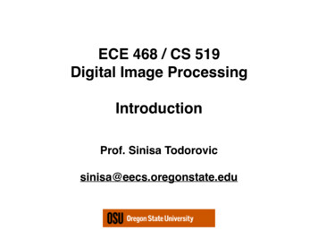
Histograms Histograms plots how many times (frequency) eachintensity value in image occursExample: Image (left) has 256 distinct gray levels (8 bits)Histogram (right) shows frequency (how many times) eachgray level occurs
Histograms Many cameras display real time histograms of sceneHelps avoid taking over‐exposed picturesAlso easier to detect types of processing previouslyapplied to image
HistogramsIntensityvalues E.g. K 16, 10 pixels have intensity value 2Histograms: only statistical informationNo indication of location of pixels
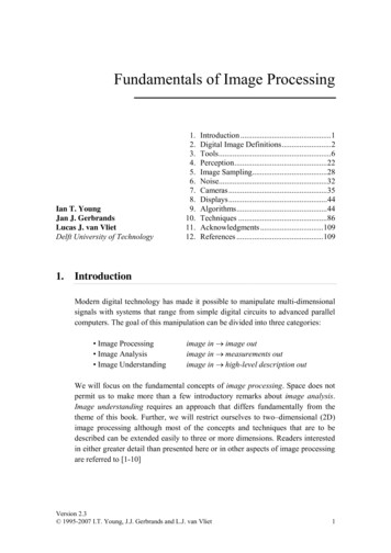
Histograms Different images can have same histogram3 images below have same histogram Half of pixels are gray, half are white Same histogram same statisicsDistribution of intensities could be differentCan we reconstruct image from histogram? No!
Histograms So, a histogram for a grayscale image with intensityvalues in rangewould contain exactly K entries E.g. 8‐bit grayscale image, K 28 256 Each histogram entry is defined as:h(i) number of pixels with intensity I for all 0 i K. E.g: h(255) number of pixels with intensity 255Formal definitionNumber (size of set) of pixelssuch that
Interpreting Histograms Log scale makes low values more visibleDifference between darkest and lightest
Histograms Histograms help detect image acquisition issuesProblems with image can be identified on histogram Over and under exposureBrightnessContrastDynamic RangePoint operations can be used to alter histogram. E.g AdditionMultiplicationExp and LogIntensity Windowing (Contrast Modification)
Image Brightness Brightness of a grayscale image is the averageintensity of all pixels in image2. Divide by total number of pixels1. Sum up all pixel intensities
Detecting Bad Exposure using HistogramsExposure? Are intensity values spread (good) out orbunched up exposed
Image Contrast The contrast of a grayscale image indicates how easilyobjects in the image can be distinguishedHigh contrast image: many distinct intensity valuesLow contrast: image uses few intensity values
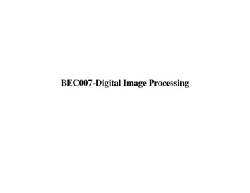
Histograms and ContrastGood Contrast? Widely spread intensity values large difference between min and max intensity valuesImageHistogramLow contrastNormal contrastHigh contrast
Contrast Equation? Many different equations for contrast existExamples: Michalson’s equation for contrast
Contrast Equation? These equations work well for simple images with 2luminances (i.e. uniform foreground andbackground)Does not work well for complex scenes with manyluminances or if min and max intensities are small
Histograms and Dynamic Range Dynamic Range: Number of distinct pixels in imageHigh Dynamic Range Low Dynamic Range(64 intensities)Extremely lowDynamic Range(6 intensity values)Difficult to increase image dynamic range (e.g. interpolation)HDR (12‐14 bits) capture typical, then down‐sample
High Dynamic Range Imaging High dynamic range means very bright and very darkparts in a single image (many distinct values)Dynamic range in photographed scene may exceednumber of available bits to represent pixelsSolution: Capture multiple images at different exposuresCombine them using image processing
Detecting Image Defects using Histograms No “best” histogram shape, depends on applicationImage defects Saturation: scene illumination values outside the sensor’s range areset to its min or max values results in spike at ends of histogramSpikes and Gaps in manipulated images (not original). Why?
Image Defects: Effect of Image Compression Histograms show impact of image compressionExample: in GIF compression, dynamic range is reducedto only few intensities ram after GIF conversionFix? Scaling image by 50% andInterpolating values recreatessome lost colorsBut GIF artifacts still visible
Effect of Image Compression Example: Effect of JPEG compression on line graphicsJPEG compression designed for color imagesOriginal histogramhas only 2 intensities(gray and white)JPEG image appearsdirty, fuzzy and blurredIts Histogram containsgray values not in original
Computing HistogramsReceives 8-bit image,Will not change itCreate array to storehistogram computedGet width and height ofimageIterate through imagepixels, add eachintensity to appropriatehistogram bin
ImageJ Histogram Function ImageJ has a histogram function ( getHistogram( ) )Prior program can be simplified if we use itReturns histogram as anarray of integers
Large Histograms: Binning High resolution image can yield very large histogramExample: 32‐bit image 232 4,294,967,296 columnsSuch a large histogram impractical to displaySolution? Binning! Combine ranges of intensity values into histogram columnsNumber (size of set) of pixelssuch thatPixel’s intensity isbetween ai and ai 1
Calculating Bin Size Typically use equal sized binsBin size? Example: To create 256 bins from 14‐bit image
Binned Histogram Create array to storehistogram computedCalculate which bin toadd pixel’s intensityIncrement correspondinghistogram
Color Image HistogramsTwo types:1. Intensity histogram: Convert colorimage to gray scale Display histogramof gray scale2. Individual ColorChannel Histograms:3 histograms (R,G,B)
Color Image Histograms Both types of histograms provide useful information aboutlighting, contrast, dynamic range and saturation effectsNo information about the actual color distribution!Images with totally different RGB colors can have same R, Gand B histogramsSolution to this ambiguity is the Combined Color Histogram. More on this later
Cumulative Histogram Useful for certain operations (e.g. histogram equalization) laterAnalogous to the Cumulative Density Function (CDF)Definition: Recursive definition Monotonically increasing Last entry ofCum. histogramTotal number ofpixels in image
Point Operations Point operations changes a pixel’s intensity value accordingto some function (don’t care about pixel’s neighbor) Also called a homogeneous operationNew pixel intensity depends on Pixel’s previous intensity I(u,v)Mapping function f( )Does not depend on Pixel’s location (u,v)Intensities of neighboring pixels
Some Homogeneous Point Operations Addition (Changes brightness) Multiplication (Stretches/shrinks image contrast range) Real‐valued functions Quantizing pixel valuesGlobal thresholdingGamma correction
Point Operation Pseudocode Input: Image with pixel intensities I(u,v) defined on[1 . w] x [1 . H]Output: Image with pixel intensities I’(u,v)for v 1 . hfor u 1 . wset I(u, v) f (I(u,v))
Non‐Homogeneous Point Operation New pixel value depends on: Old value pixel’s location (u,v)
Clamping Deals with pixel values outside displayable range If (a 255) a 255;If (a 0) a 0;Function below will clamp (force) all values to fallwithin range [a,b]
Example: Modify Intensity and Clamp Point operation: increase image contrast by 50%then clamp values above 255Increase contrastby 50%
Inverting Images 2 steps1.2. Multiple intensity by ‐1Add constant (e.g. amax)to put result in range[0,amax]Implemented asImageJ methodinvert( )OriginalInverted Image
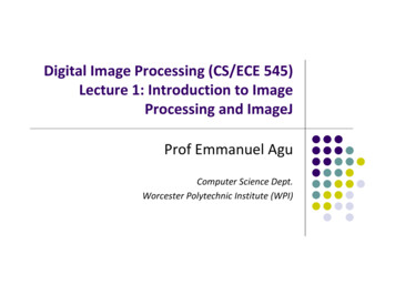
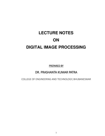
Images taken from Gonzalez & Woods, Digital Image Processing (2002)Image Negatives (Inverted Images) Imagenegatives useful for enhancing white orgrey detail embedded in dark regions of an image OriginalImageNote how much clearer the tissue is in the negativeimage of the mammogram belows 1.0 - rNegativeImage
Thresholding Implemented as imageJ method threshold( )
Thresholding Example
Thresholding and Histograms Example with ath 128 Thresholding splits histogram, merges halves into a0 a1
Images taken from Gonzalez & Woods, Digital Image Processing (2002)Basic Grey Level Transformations 3 most common gray level transformation: Linear Logarithmic Negative/IdentityLog/Inverse logPower law nth power/nth root
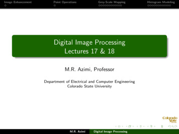
Logarithmic Transformations Mapsnarrow range of input levels wider range ofoutput values Inverse log transformation does opposite transformation The general form of the log transformation isNew pixel valueOld pixel values c * log(1 r) Log transformation of Fourier transform shows more details log(1 r)
Images taken from Gonzalez & Woods, Digital Image Processing (2002)Power Law Transformations Powerlaw transformations have the formPowerγs c*rOld pixel valueNew pixel valueConstant Mapnarrow range ofdark input values intowider range of outputvalues or vice versa Varyingγ gives a wholefamily of curves
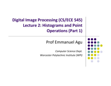
Power Law Example MagneticResonance(MR) image of fracturedhuman spine Differentpower valueshighlight differentdetailss r 0.6s r 0.4Images taken from Gonzalez & Woods, Digital Image Processing (2002)Original
Intensity Windowing A clamp operation, then linearly stretching imageintensities to fill possible rangeTo window an image in [a,b] with max intensity M
Intensity Windowing ExampleContrastseasier to see
Point Operations and Histograms Effect of some point operations easier to observe on histograms Increasing brightnessRaising contrastInverting imagePoint operations only shift, merge histogram entriesOperations that merge histogram bins are irreversibleCombining histogramoperation easier toobserve on histogram
Automatic Contrast Adjustment Original intensity rangeIf amin 0New intensity rangeandamax 255
Effects of Automatic Contrast AdjustmentLinearly stretchingrange causes gapsin histogramOriginalResult of automaticContrast Adjustment
Modified Contrast Adjustment
Histogram Equalization Adjust 2 different images to make their histograms(intensity distributions) similarApply a point operation that changes histogram ofmodified image into uniform distributionHistogramCumulativeHistogram
Histogram EqualizationSpreading out the frequencies in an image (orequalizing the image) is a simple way to improve darkor washed out imagesCan be expressed as a transformation of histogram rk: input intensitysk: processed intensityk: the intensity range(e.g 0.0 – 1.0)processed intensitysk T (rk )Intensity range(e.g 0 – 255)input intensity
Images taken from Gonzalez & Woods, Digital Image Processing (2002)Equalization Transformation Function
Images taken from Gonzalez & Woods, Digital Image Processing (2002)Equalization Transformation FunctionsDifferent equalization function (1‐4) may be used
Images taken from Gonzalez & Woods, Digital Image Processing (2002)Equalization Examples1
Images taken from Gonzalez & Woods, Digital Image Processing (2002)Equalization Examples2
Images taken from Gonzalez & Woods, Digital Image Processing (2002)Equalization Examples34
References Wilhelm Burger and Mark J. Burge, Digital ImageProcessing, Springer, 2008 Histograms (Ch 4)Point operations (Ch 5)University of Utah, CS 4640: Image Processing Basics,Spring 2012Rutgers University, CS 334, Introduction to Imagingand Multimedia, Fall 2012Gonzales and Woods, Digital Image Processing (3rdedition), Prentice Hall
Image negatives useful for enhancing white or grey detail embedded in dark regions of an image Note how much clearer the tissue is in the negative image of the mammogram below s 1.0 - r Original Image Negative Images taken from Gonzalez & W Image oods, Digital Image Processing (2002)