Transcription
Factor Analysis (Chpater 13)Factor analysis is a dimension reduction technique where the number ofdimensions is specified by the user. The idea is that there are underlying“latent” variables or “factors”, and several variables might be measures ofthe same factor. Here the original variables are considered to be linearcombinations of the underlying factors.The idea is that the number of factors might be lower than the number ofvariables, and might correspond to theories about the data. For example,you might think there are different cognitive abilities, such as spatialreasoning, analytic reasoning, analogical reasoning, quantitative ability,linguistic ability, etc. A test might have 100 questions that measure theseunderlying abilities, so different linear combinations of the factors mightgive the distribution of the answers on the different test questions.April 24, 20151 / 67
Factor analysisVariables that are closely related to each other should have relatively highcorrelation, and variables that are not closely related should have relativelylow correlation. Looking at correlations between variables, the idealcorrelation matrix might look like this 1.00 0.90 .05 .05 .05 .90 1.00 .05 .05 .05 .05 .05 1.00 .90 .90 .05 .05 .90 1.00 .90 .05 .05 .05 .90 1.00For this matrix, the first two variables are high correlated with each otherbut to no other variables, and similarly the last three variables are highlycorrelated to each other but to no other. Thus, the data could plausiblyhave arisen if there were two factors, with variables 1 and 2 measuring thefirst factor and variables 3–5 measuring the second factor.April 24, 20152 / 67
Factor analysisFactor analysis is similar to principal components in that linearcombinations are used for dimension reduction. However1. In factor analysis, the original variables are linear combinations of thefactors. principal components are linear combinations of the originalvariables.2. principal componentsseeks to find linear combinations to explain thePtotal variance i si2 , whereas factor analysis tries to account forcovariances in the data3. Factor analysis is somewhat controversial among statisticians partlybecause solutions are not unique.April 24, 20153 / 67
Factor analysisIn factor analyis, we treat data as arising from a single factor. We assumethat there arep variables and m p factors, where m is fixed in advance.The factors can be represented by f1 , . . . , fm . Then for obervation yi , themodel isy1 µ1 λ11 f1 λ12 f2 · · · λ1m fm ε1y2 µ2 λ21 f1 λ21 f2 · · · λ2m fm ε2.yp µp λp1 f1 λp1 f2 · · · λpm fm εpThis would look very similar to a regression model if we moved the µs tothe right hand sides, except that the factor loadings, λij are individualizedfor each subject, and the factors are unobserved. Also, for eachobservation, we have p equations rather than one equation per observationthat we would normally have in regression.April 24, 20154 / 67
Factor analysisThe factor loading λij indicates the importance of factor j to variable i.For example, if λi2 is large for variables 1–3 and small for variables 4–p,the factor 2 is important for the first three variables but less important forthe remaining variables. Hopefully this has some interpretation where theresearcher hopes that they can describe something that relates the firstthree variables but not the remaining ones.Although the factors are unknown, they are also considered randomvariables, and in the model we haveE (fi ) 0,Var (fi ) 1,Cov (fi , fj ) 0So the factors are assumed to be independent. The model also assumesE (εi ) 0,Var (εi ) ψiIn other words, the error terms are allowed to differ for each variable. Inaddition, it is assumed that Cov (εi , fj ) 0 and Cov (εi , εj ) 0.April 24, 20155 / 67
Factor analysisBased on the assumptions,Var (yi ) λ2i1 λ2i2 · · · λ2im ψiApril 24, 20156 / 67
Factor analysisThe model can also be written in matrix notation asy µ Λf εwhere y (y1 , . . . , yp )0 , µ (µ1 , . . . , µp )0 , f (f1 , . . . , fm )0 ,ε (ε1 , . . . , εp )0 and Λ (λij ) with i 1, . . . , p, j 1, . . . , m.Because µ is a constant, the covariance matrix isVar (y) Cov (Λf ε) Cov (Λf) Cov (ε) ΛIΛ0 Ψ ΛΛ0 ΨWhere Ψ diag(ψ1 , . . . , ψp ).April 24, 20157 / 67
Factor analysis: example with 5 variables, 2 factorsApril 24, 20158 / 67
Factor analysisWe can interpret the matrix Λ as the covariances between the variablesand the factorsΛ Cov (y, f)If the variables are standardized (using z-scores), then λi,j is thecorrelation between the ith variable and jth factor.The variance of a variable can be partitioned into a portion due to thefactors and the remaining portion,Var (yi ) σii (λ2i1 · · · λip 2 ) ψi hi2 ψiHere hi2 is called the comunality or common variance and ψ is called thespecific variance or residual variance.April 24, 20159 / 67
Factor analysisThe hope in factor analysis is thatΛΛ0 Ψ Σ,the covariance matrix for the original data, but often the approximation isnot very good if there are too few factors. If the estimated factor analysisstructure doesn’ fit the estimate for Σ, this indicates the inadequacy ofthe model and suggests that more factors might be needed.The book points out that this can be a good thing in that the inadequacyof the model might be easier to see than other statistical settings thatrequire complicated diagnostics.April 24, 201510 / 67
Factor analysisAn issue that bothers some is that the factor loadings are not unique. If Tis any othogonal matrix, then TT0 I. Consequently,y µ ΛTT0 f εis equivalent to the model with TT0 removed, and factor loadings ΛT withfactors T0 f will give equivalent results, and the new model could be writteny µ Λ f εwith Λ ΛT and f T0 f.The new factors and factor loadings are different, but the communalitiesand residual variances are not affected.April 24, 201511 / 67
Factor analysisThere are different ways to estimate the factor loadings Λ. The first iscalled the principal component method, but is unrelated to principalcomponents (!). Four methods listed in the book are1. “Princpal components” (not PCA)2. Principal factors3. Iterated principal factors4. maximum likelihoodApril 24, 201512 / 67
Factor analysisFor the first approach, the idea is to initially factor S, the samplecovariance matrix of the data, into0bΛbS Λusing singular value decomposition, so that0S CDC0 CD1/2 D1/2 C (CD1/2 )(CD1/2 )0where C is an orthogonal matrix with normalized eigenvectors and D is adiagonal matrix of eigenvalues θ1 , . . . , θp . θ is used rather than λ becauseλ is used for the factor loadings (not sure why).b to be p mHere CD1/2 is p p but we want ΛApril 24, 201513 / 67
Factor analysisTo get a matrix with the right dimensions, we use the first m columns ofb assuming that θ1 · · · θm and the columns of CCD1/2 to define Λ,correspond to the eigenvectors with nonincreasing eigenvalues (i.e.,rearrange columns of C and D if necessary).bΛb 0 from S:To estimate Ψ, we subtract the ith diagonal of Λψbi sii mXb2λijj 1b 0 . Then the ijth element of ΛbΛb 0 isTo confirm that this is right, let A ΛmXk 1λik akj mXλik λjkk 1For the diagonal, j i, and we have λ2ik in the summand, and the bookuses j instead of k as the index.April 24, 201514 / 67
Factor analysisbΛb 0 only approximate S. Adding ΨbThe fact that m p is what makes Λmeans that the original sample variances are recovered exactly in themodel but that the covariances are still estimated.The estimated communality for variable i is the sum of the estimatedfactor loadings for that variable:bhij mXb2λijj 1The estimated variance due to the jth factor ispXb 2 θjλiji 1bwhich is the sum of squares of the ith column of Λ.April 24, 201515 / 67
Factor analysisThis equivalence is due to the followingpXi 1b2 λijppXX 2( θj cij ) θjcij2 θji 1i 1where c1j , . . . , cpj is the jth normalized eigenvector.April 24, 201516 / 67
Factor analysisThe proportion of the total sample variance (adding the variances of allvariables separately, regardless of covariances), is thereforePpb2i 1 λijtr(S) θjtr(S)Note that if variables are standardized, then in place of the covariancematrix S we use the correlation matrix R, in which case the denominator isp.The fit of the model can be measured by comparing the covariance matrixwith its estimate into an error matrixbΛb 0 Ψ)bE S (ΛApril 24, 201517 / 67
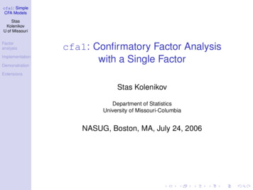
Factor analysis: example with 5 variables, 7 observationsApril 24, 201518 / 67
Factor analysisThe eigenvalues of the correlation matrix are3.2631.5380.1680.0310indicating that there is collinearity in the columns (they are not linearlyindependent). The proportion of the variance explained by the first factoris 3.263/5 0.6526 and the proportion explained by the first two togetheris (3.263 1.538)/5 0.9602, meaning that two factors could account for96% of the variability in the data. Looking at the correlation matrix, wehave strong positive correlations within the sets {Kind, Happy , Likeable}and {Intelligent, Just}, suggesting that these could correspond to separateand somewhat independent factors in the characteristics perceived inpeople by the subject.April 24, 201519 / 67
Factor analysis: example with 5 variables, 7 observationsApril 24, 201520 / 67
Factor analysisApril 24, 201521 / 67
Factor analysisIn the example, the loadings in the first column give the relativeimportance of the variables for factor 1, while the loadings in the secondcolumn give the relative importance of factor 2. For factor 1, the highestvariables are for Kind and Happy, with Likeable being third. The Justvariable is somewhat similar to the Happy variable. For factor 2, Intelligentand Just stand out as having much higher correlations than the othervariables.As mentioned previously it is possible to rotate the factor loadings,however. The book points out that you could rotate the loadings (orequivalently, rotate the factors themselves). Plotting the factor loadingson a two-dimensional plot, we can see how to rotate the data to make aclearer (more easily interpretable) contrast between the factors. This isdone by choosing T to be a suitable rotation matrix.April 24, 201522 / 67
Factor analysisApril 24, 201523 / 67
Factor analysisSince there is no unique way to rotate the factors, there is no unique wayto interpret the factor loadings. So, for example, variables 3 and 5 aresimilar on the original factor 1 (but not factor 2), while on the rotatedfactors, variables 3 and 5 are quite different, with variable 5 being high onfactor 2 and variable 3 being high on factor 1. It seems that you couldchoose whether or not to rotate axes depending on the story you want totell about variable 3.The book suggests that when the factors are rotated, the factors could beinterpreted as representing humanity (rotated factor 1) and rationality(factor 2). An objection is that this is imposing a theory of preconceivedpersonalities onto the data.April 24, 201524 / 67
Factor analysisAnother approach called the principle factor method is to estimate factorb and then useloadings is to first estimate Ψb ΛbΛbS Ψor00b ΛbΛbR ΨHerebR Ψcan be approximated using rij , the sample correlations, for the off diagonalelements. For the diagonals, these can be estimated using Ri2 , the squaredmultiple correlation between yi and the remaining variables. This iscomputed as1bhi Ri2 1 iiriiwhere r denotes the ith diagonal element of R 1 .April 24, 201525 / 67
Factor analysisUsing S instead of R is similar withwidehathii2 sii 1s iiThese approaches assume that R or S are nonsingular. Otherwise, hi2 canbe estimated using the largest correlation in the ith row of R.b can be estimated using singular valueOnce R Ψ is estimated, Λb is the jthdecomposition. The sum of squares of the jth column of Λeigenvalue of R Ψ, and the sum of squares of the ith row of R Ψ ishi2 , the communality.April 24, 201526 / 67
Factor analysisbThe principal factor method can be iterated to improve estimates. Once Λis given, this can be used to get improved estimates of the communalities,hi2 asmX2bb2hi λiji 1b is given by. Then an updated estimate for Ψψbi rii bhi2using the updated value for bhi2 .April 24, 201527 / 67
Factor analysisThe three methods — principal components, principal factors, and iteratedprincipal factors — give similar results if the correlations are large and m issmall, and if the number of variables p is large. Apparently, the iterativeapproach can result in an estimated commonality of greater than 1, whichcorresponds to a ψ value (a variance) being negative. Different softwaremight handle this differently, either reporting an error or truncatingestimates of commonalities to 1.April 24, 201528 / 67
Factor analysisMaximum likelihood can be done, but assumes a particular distribution forthe variables, which is typically multivariate normal, which is ofteninappropriate for the types of data to which factor analysis is usuallyapplied. This approach is also difficult numerically and requires iterativeprocedures to approximate the maximum liklelihood solution, and theseprocedures are not guaranteed to work (they might fail to converge).April 24, 201529 / 67
Factor analysisThe number of factors might either correspond to a hypothesis about thevariables related to the data or some method can be used. Here are somestrategies:1. choose enough factors so that the percentage of variance accountedfor,Pmi 1 θitr(R)is sufficiently large, e.g., 90%2. choose m to be the number of eigenvalues greater than the averageeigenvalue3. make a scree plot of the eigenvalues4. If using likelihood, do a likelihood ratio test ofH0 : Σ ΛΛ0 Ψ, H1 : Σ 6 ΛΛ0 ΨApril 24, 201530 / 67
Factor analysisBecause the choice of m might not be obvious, there is a danger that aresearcher will choose m to fit a theory about how many factors and whichfactors are needed to explain the data. This is also a potential danger withprincipal components or MDS, where a researcher might want to claimthat genes correlate with geography for example, and use only twodimensions without testing whether three dimensions would be moreappropriate for the data.April 24, 201531 / 67
Factor analysisWe mentioned earlier that factors can be rotated. This can be donevisually, using trial and error to get an approximate rotation, or a rotationcan be try to optimize some quantity. Varimax is an optimizationtechnique that rotates the data so that the squared factor loadings areeither minimized (close to 0) or maximized, so that variables are eitherstrongly associated with a factor or fairly unrelated to a factor. This canbe applied in two or more dimensions.Another approach is called oblique rotation, in which the factors aremade to not be orthogonal. In this case, instead of using an orthogonaltransformation matrix T, a nonorthogonal matrix Q is used instead, sothat the new factors are f Q0 f. If this was applied to the personalitydata, it would imply that the factors of humanity and rationality (orlogicalness) are not independent.April 24, 201532 / 67
Factor analysisApril 24, 201533 / 67
Factor analysisbij is statistically signficant. AIt is difficult to say whether a factor loading λthreshold of 0.3 has been advocated in the past, but the author arguesthat this is often too low and can result models being difficult to interpret.The book suggests that 0.5 or 0.6 is more useful to consider a factorloading large, although a good threshold also depends on the number offactors, m, with larger m tending to result in smaller factor loadings.April 24, 201534 / 67
Factor analysisIt is also possible to estimate factors related to a given observation. Theseare called factor scores,fi (bfi , bf2 , . . . , bfm )0where i 1, . . . , n. These estimate the factor values for each observation.The factor scores can be used to understand the observations themselvesor are sometimes as input to MANOVA.The factor scores are modeled as functions of the original observationsfi B01 (yi y) where B1 (βij ) is a matrix of regression coefficients and is an errorterm (distinguished from ε used for the factor analysis model).April 24, 201535 / 67
Factor analysisThe n equations for fi can be combined asApril 24, 201536 / 67
Factor analysisThe model essentially looks like a multivariate regression model with Yc(the centered version of Y) as the design matrix and F in place of Y (thematrix of responses in a usual regression). An important difference here isthat F is unobserved.If F had been observed, then the estimate for B1 would be (using theusual matrix representation of regression)b 1 (Y0 Y) 1 Yc FBcApril 24, 201537 / 67
Factor analysisIn multivariate regression (which we skipped over in chapter 10), you canestimate B1 asb 1 S 1 SxyByywhere Sy y is the usual covariance matrix S and Sxy represents covariancesbetween the explanatory variables and response variables, so in our case isbcov (f, y) Λ.We can estimate F byb Yc S 1 ΛbF(or use R in place of S). Often you would obtain factor scores after doingrotations.April 24, 201538 / 67
Factor analysisAn example from the book:April 24, 201539 / 67
Factor analysisThere were 20 voices read to 30 judges who judged the voices on a 14point scale on the following variables: intelligent, ambitious, polite, active,confident, happy, just, likeable, kind, sincere, dependable, religious,good-looking, sociable, and strong. The results from the 30 judges werethen averaged, so that there were 20 observations and 15 variables.Note that in a mixed-model framework, you could use the original 30judges separate scores, so that you would have 600 observations, but therewould be correlation in the data so that scores from the same judge aremore likely to be similar. You could also model this using multivariateregression just using the judges as blocks. In mixed models, we think ofthere being random effects for the judges, who have been selected fromsome larger population of possible judges.April 24, 201540 / 67
Factor analysis: from the bookApril 24, 201541 / 67
Factor analysisThe eigenvalues are 7.91, 5.85, .31, .26, . . . , .002. Since only the first twoeigenvalues are large, this suggests that two factors is reasonable for thedata. This can be visualized by a scree plot.April 24, 201542 / 67
Factor analysisApril 24, 201543 / 67
Factor analysisApril 24, 201544 / 67
Factor analysisApril 24, 201545 / 67
Factor analysisAs a general interpretation, the researchers categorized the factors asrepresenting benevolence and competence, which you might question.Different researchers might have used different words to describe thesegroupings of variables. Slower voices were perceived to be more“benevolent” but less “competent”, and faster voices were perceived to bemore “competent” but less “benevolent”.April 24, 201546 / 67
Factor analysisThe author points out that many statisticians dislike factor analysis partlybecause of the nonuniqueness of the factor rotations and that this couldlead to different interpretations. One question is whether the factors reallyexist? The previous example seems to suggest that people judge othersaccording to their perceived benevolence or competence. It would havebeen interesting if these questions had been asked in addition to theattributes such as strength, intelligence, kindness, etc.April 24, 201547 / 67
Factor analysisApril 24, 201548 / 67
Factor analysisA suggestion in the book for determining whether the factors aremeaningful is to use replication – either by replicating the study itself or bysplitting the data in half and seeing if the same factors seem to emerge forthe two halves of the data. A difficult with this is that factor analysis isoften applied in cases where there aren’t many observations. The bookalso points out that “there are many data sets for which factor analysisshould not be applied”.April 24, 201549 / 67
Factor analysis in RThere are a few ways to do factor analysis in R. Some common ones arethe fa() and factanal() functions. The fa() function is in the psychpackage. factanal() is built into R but only does maximum likelihoodfactor analysis.The fa() function is more flexible, for example, it can handle missing data(which would be common in questionnaire data) and doesn’t only domaximum likelihood, as well as having more options.April 24, 201550 / 67
Factor analysis in Rfa(r,nfactors 1,n.obs NA,n.iter 1, rotate "oblimin", scores "regreresiduals FALSE, SMC TRUE, covar FALSE,missing FALSE,impute "median"min.err 0.001, max.iter 50,symmetric TRUE, warnings TRUE, fm "malpha .1,p .05,oblique.scores FALSE,np.obs,use "pairwise",cor "cor",The input is either a correlation matrix, covariance matrix, or the original datamatrix. The user specifies the number of factors. The number of observations(number of rows in original data, not the number of variables or number of rowsin the correlation matrix) must be specified to get confidence intervals andgoodness-of-fit statistics.There are a surprising number of algorithms to do the rotations, includingrotate: "none", "varimax", "quartimax", "bentlerT", "equamax","varimin", "geominT" and "bifactor" are orthogonal rotations."promax", "oblimin", "simplimax", "bentlerQ, "geominQ"April 24, 201551 / 67
Factor analysis in Rn.iter specifies the number of iterations to get bootstrapped confidenceintervals for factor loadings. If there is only one iteration, then confidenceintervals aren’t obtained. fm specifies the method for doing the factoranalysis, with choices including minres for Ordinary Least Squares, wlsfor Weighted Least Squares. ml for maximum likelihood, pa does principalfactor rotation (one of the methods in class) and so on.April 24, 201552 / 67
ExampleThe following is an example questionnaire data set with 42 questionsasking subjects to rate a web site on different variables. A guideline for thevariables is the following:TTU Website "ease of finding information""web design""attitude toward TTU""attitude toward web site"April 24, 201553 / 67
Questions:Q1 Finding information on athleticsQ2 Finding information on on-campus housingQ3 Finding information on extracurricular activities (clubs)Q4 Finding information on admissions (fees, general, etc.)Q5 Finding information on financial aid and scholarship programsQ6 Finding information on majors/minorsQ7 Finding information on student life (social life)Q8 Finding information on directions (maps)Q9 Finding information on admissions criteriaQ10 The use of graphics and pictures was favorable.Q11 The download speed frustrated me.Q12 The color coordination was pleasant.Q13 The virtual tour was valuable. (If applicable).Q14 I was unable to clearly read the web site’s text.Q15 The search function was worthless.Q16 I did not think this web site was unique in appearance and conteQ17 I liked the design of the home page.April 24, 201554 / 67
Q18 Do you believe this web site provided entertainment value?Q19 Do you believe this web site has a friendly tone?Q20 I am attracted to web sites that have a friendly tone.Q21 I prefer for a college/university website to be entertaining.Q22 Ordinary:Exceptional ProductQ23 Not at all high quality:Extremely high qualityQ24 Poor value:Excellent ValueQ25 Boring:ExcitingQ26 Not a worthwhile university:A worthwhile universityQ27 Unappealing university:Appealing universityQ28 I would not recommend this university:I would recommend this universityQ29 I would not apply to this university:I would applyto this universityQ30 This website makes it easy for me to build arelationship with this university.Q31 I would like to visit this website again in the future.Q32 I’m satisfied with the information provided by this web site.April 24, 201555 / 67
Q33 I feel comfortable in surfing this web site.Q34 I feel surfing this web site is a good way for me to spend my tiQ35 Compared with other university web sites, I would rate this oneOne of the best:One of the worstQ36 Would you apply to this university?Q37 Would you recommend a friend, family member,or peer to apply to this university?Q38 Please indicate your gender.Q39 Please indicate your ethnicity.Q40 Are you currently enrolled at a university, college,trade school, etc.?Q41 If you answered yes, please indicate your classificationQ42 If you are a student, are you considering to transfer?April 24, 201556 / 67
ExampleThe data is in a comma delimited file, and looks something like ,2,1,1,2,3,Note that there is missing data when two commas appear in a row.April 24, 201557 / 67
ExampleThe questionnaire was designed with four themes in mind in the first 35questions: ease of using the website, web design, attitude toward theschool, and attitutde toward the web site, so it is plausible that that thereare three factors largely influencing the responses. x - read.table("http://math.unm.edu/ james/ttu websurv.csv",sep ",",header T) survey - x[,1-35] library(psych) a - fa(survey,nfactors 4,rotate "varimax",fm "pa") summary(a)actor analysis with Call: fa(r survey, nfactors 4, rotate "varTest of the hypothesis that 4 factors are sufficient.The degrees of freedom for the model is 662 and the objective functThe number of observations was 328 with Chi Square 1408.51 witThe root mean square of the residuals (RMSA) is 0.05The df corrected root mean square of the residuals is0.06April 24,201558 / 67
ExampleTo get an idea of the number of factors, one can look at the eigenvalues: names(a)[1] "residual"[4] "nh"[7] "crms"[10] "fit"[13] "factors"[16] "objective"[19] "PVAL"[22] "null.dof"[25] "RMSEA"[28] "r.scores"[31] "score.cor"[34] "communality"[37] "e.values"[40] "Structure"[43] pril 24, 201559 / 67
a e.values[1] 8.7740074 2.5751451 2.1574631 1.8840962[8] 1.2640660 1.1430268 1.1205339 1.1069691[15] 0.8568173 0.8539552 0.8063560 0.7693574[22] 0.6675796 0.6449242 0.6134014 0.5843541[29] 0.4661804 0.4492236 0.4361704 0.3815501[36] 0.2869011 0.2764981 0.2549595 0.2340578 cumsum(a e.values)/sum(a e.values)[1] 0.2140002 0.2768086 0.3294296 0.3753832[8] 0.5156637 0.5435424 0.5708725 0.5978717[15] 0.6907341 0.7115623 0.7312295 0.7499943[22] 0.8182225 0.8339523 0.8489133 0.8631659[29] 0.9110939 0.9220506 0.9326889 0.9419950[36] 0.9737798 0.9805236 0.9867422 .80.9April 24, 201560 / 67
ExampleA common test is to use the number of factors where the eigenvalues are greaterthan 1, but this would require 12 factors, and you need 21 factors to explain 80%of the variance, so this is not good. It means that the data will be very hard tointerpret in terms of latent variables or factors. On the other hand, it means thatthe questionnaire is asking different questions and not just asking the samequestion 10 different ways.To see some of the other output, the factor analysis gives linear combinations ofthe factors for each question. aFactor Analysis using method paCall: fa(r survey, nfactors 4, rotate "varimax", fm "pa")Standardized loadings (pattern matrix) based upon correlation matrixPA1PA2PA3PA4h2u2 comQ10.17 -0.12 0.31 0.45 0.342 0.66 2.3Q20.09 -0.05 0.40 0.02 0.169 0.83 1.2Q30.13 -0.23 0.51 -0.11 0.342 0.66 1.7Q40.12 0.00 0.50 0.25 0.328 0.67 1.6April 24, 201561 / 67
ExampleEven though four factors doesn’t fit the data well, we can try to see if wecan interpret the factors to some extent. The factor loadings can be madeeasier to read by only printing those above a certain threshold: print(a loadings,cutoff .5)April 24, 201562 / 67
5Q16Q17Q18Q19PA3PA40.5060.5360.515-0.529April 24, 201563 / 67
Repeating the factor analysis with more factors can show some moregroupings of questions, and can change the groupings of the variables.If your interest is more in redesigning the survey (for example, in order toask fewer questions), this can still be a useful tool, even if you are notfiguring out the number of factors or being able to interpret the factorsvery easily.April 24, 201564 / 67
50.6280.5130.5090.6270.5950.605April 24, 201565 / 67P
Structural Equation ModelingStructural equation modeling is a topic that we won’t go into, but isrelated to factor analysis. Confirmatory factory analysis (where you t
Factor Analysis (Chpater 13) Factor analysis is a dimension reduction technique where the number of dimensions is speci ed by the user. The idea is that there are underlying \latent" variables or \factors", and several variables might be measures of the same factor. Here the original variables are considered to be linear